Download
1 / 59
650 likes | 961 Views
Exploratory Data Analysis: One Variable. FPP 3-6. Plan of attack. Distinguish different types of variables Summarize data numerically Summarize data graphically Use theoretical distributions to potentially learn more about a variable. The five steps of statistical analyses.

E N D
Plan of attack • Distinguish different types of variables • Summarize data numerically • Summarize data graphically • Use theoretical distributions to potentially learn more about a variable.
The five steps of statistical analyses • Form the question • Collect data • Model the observed data • We start with exploratory techniques. • Check the model for reasonableness • Make and present conclusions
Just to make sure we are on the same page • More (or repeated) vocabulary • Individuals are the objects described by a set of data • examples: employees, lab mice, states… • A variable is any characteristic of an individual that is of interest to the researcher. Takes on different values for different individuals • examples: age, salary, weight, location… • How is this different from a mathematical variable?
Just to make sure we are on the same page #2 • Measurement The value of a variable obtained and recorded on an individual • Example: 145 recorded as a person’s weight, 65 recorded as the height of a tree, etc. • Data is a set of measurements made on a group of individuals • The distribution of a variable tells us what values it takes and how often it takes these values
Two Types of Variables • a categorical/qualitative variable places an individual into one of several groups or categories • examples: • Gender, Race, Job Type, Geographic location… • JMP calls these variables nominal • a quantitative variable takes numerical values for which arithmetic operations such as adding and averaging make sense • examples: • Height, Age, Salary, Price, Cost… • Can be further divided to ordinal and continuous • Why two types? • Both require their own summaries (graphically and numerically) and analysis. • I can’t emphasis enough the importance of identifying the type of variable being considered before proceeding with any type of statistical analysis
Example • Age: quantitative • Gender: categorical • Race: categorical • Salary: quantitative • Job type: categorical
Variable types in JMP • Qualitative/categorical • JMP uses Nominal • Quantitative • Discrete • JMP uses Ordinal • Continuous • JMP uses Continuous
Exploratory data analysis • Statistical tools that help examine data in order to describe their main features • Basic strategy • Examine variables one by one, then look at the relationships among the different variables • Start with graphs, then add numerical summaries of specific aspects of the data
Exploratory data analysis: One variable • Graphical displays • Qualitative/categorical data: bar chart, pie chart, etc. • Quantitative data: histogram, stem-leaf, boxplot, timeplot etc. • Summary statistics • Qualitative/categorical: contingency tables • Quantitative: mean, median, standard deviation, range etc. • Probability models • Qualitative: Binomial distribution(others we won’t cover in this class) • Quantitative: Normal curve (others we won’t cover in this class)
Summary table • we summarize categorical data using a table. Note that percentages are often called Relative Frequencies.
Bar graph • The bar graph quickly compares the degrees of the four groups • The heights of the four bars show the counts for the four degree categories
Pie chart • A pie chart helps us see what part of the whole group forms • To make a pie chart, you must include all the categories that make up a whole
Summary of categorical variables • Graphically • Bar graphs, pie charts • Bar graph nearly always preferable to a pie chart. It is easier to compare bar heights compared to slices of a pie • Numerically: tables with total counts or percents
Quantitative variables • Graphical summary • Histogram • Stemplots • Time plots • more • Numerical sumary • Mean • Median • Quartiles • Range • Standard deviation • more
Histograms The bins are: 3.0 ≤ rate < 4.0 4.0 ≤ rate < 5.0 5.0 ≤ rate < 6.0 6.0 ≤ rate < 7.0 7.0 ≤ rate < 8.0 8.0 ≤ rate < 9.0 9.0 ≤ rate < 10.0 10.0 ≤ rate < 11.0 11.0 ≤ rate < 12.0 12.0 ≤ rate < 13.0 13.0 ≤ rate < 14.0 14.0 ≤ rate < 15.0
Histograms The bins are: 3.0 ≤ rate < 4.0 4.0 ≤ rate < 5.0 5.0 ≤ rate < 6.0 6.0 ≤ rate < 7.0 7.0 ≤ rate < 8.0 8.0 ≤ rate < 9.0 9.0 ≤ rate < 10.0 10.0 ≤ rate < 11.0 11.0 ≤ rate < 12.0 12.0 ≤ rate < 13.0 13.0 ≤ rate < 14.0 14.0 ≤ rate < 15.0
Histograms The bins are: 2.0 ≤ rate < 4.0 4.0 ≤ rate < 6.0 6.0 ≤ rate < 8.0 8.0 ≤ rate < 10.0 10.0 ≤ rate < 12.0 12.0 ≤ rate < 14.0 14.0 ≤ rate < 16.0 16.0 ≤ rate < 18.0
Histograms • Where did the bins come from? • They were chosen rather arbitrarily • Does choosing other bins change the picture? • Yes!! And sometimes dramatically • What do we do about this? • Some pretty smart people have come up with some “optimal” bin widths and we will rely on there suggestions
Histogram • The purpose of a graph is to help us understand the data • After you make a graph, always ask, “What do I see?” • Once you have displayed a distribution you can see the important features
Histograms • We will describe the features of the distribution that the histogram is displaying with three characteristics • Shape • Symmetric, skewed right, skewed left, uni-modal, multi-modal, bell shaped • Center • Mean, median • Spread (outliers or not) • Standard deviation, Inter-quartile range
Incomes from 500 households in 2000 current population survey
Histogram vs. Bar graph • Spaces mean something in histograms but not in bar graphs • Shape means nothing with bar graphs • The biggest difference is that they are displaying fundamentally different types of variables
Time Plots • Many variables are measured at intervals over time • Examples • Closing stock prices • Number of hurricanes • Unemployment rates • If interest is a variable is to see change over time use a time plot
Time Plots • Patterns to look for • Patterns that repeat themselves at known regular intervals of time are called seasonal variation • A trend is a persistant, long-term rise or fall
Time plots number of hurricanes each year from 1970 - 1990
Numerical summaries of quantitative variables • Want a numerical summary for center and spread • Center • Mean • Median • Mode • Spread • Range • Inter-quartile range • Standard deviation • 5 number summary is a popular collection of the following • min, 1st quartile, median, 3rd quartile, max
Mean • To find the mean of a set of observations, add their values and divide by the number of observations • equation 1: • equation 2:
Mean example • The average age of 20 people in a room is 25. A 28 year old leaves while a 30 year old enters the room. • Does the average age change? • If so, what is the new average age?
Median • The median is the midpoint of a distribution • The number such that half the observations are smaller and the other half are larger • Also called the 50th percentile or 2nd quartile • To compute a median • Order observations • If number of observations is odd the median is the center observation • If number of observations is even the median is the average of the two center observations
Median example • The median age of 20 people in a room is 25. A 28 year old leaves while a 30 year old enters the room. • Does the median age change? • If so, what is the new median age? • The median age of 21 people in a room is 25. A 28 year old leaves while a 30 year old enters the room. • Does the median age change? • If so, what is the new median age?
Mean vs Median • When histogram is symmetric mean and median are similar • Mean and median are different when histogram is skewed • Skewed to the right mean is larger than median • Skewed to the left mean is smaller than median • The business magazine Forbes estimates that the “average” household wealth of its readers is either about $800,000 or about $2.2 million, depending on which “average” it reports. Which of these numbers is the mean wealth and which is the median wealth? Why?
Mean vs Median • Symmetric distribution
Mean vs Median • Right skewed distribution
Mean vs Median • Left skewed distribution
Extreme example • Income in small town of 6 people $25,000 $27,000 $29,000 $35,000 $37,000 $38,000 • Mean is $31,830 and median is $32,000 • Bill Gates moves to town $25,000 $27,000 $29,000 $35,000 $37,000 $38,000 $40,000,000 • Mean is $5,741,571 median is $35,000 • Mean is pulled by the outlier while the median is not. The median is a better of measure of center for these data
Is a central measure enough? • A warm, stable climate greatly affects some individual’s health. Atlanta and San Diego have about equal average temperatures (62o vs. 64o). If a person’s health requires a stable climate, in which city would you recommend they live?
Measures of spread • Range: • subtract the largest value form the smallest • Inter-quartile range: • subtract the 3rd quartile from the 1st quartile • Standard Deviation (SD): • “average” distance from the mean • Which one should we use?
Standard Deviation • The standard deviation looks at how far observations are from their mean • It is the square root of the average squared deviations from the mean • Compute distance of each value from mean • Square each of these distances • Take the average of these squares and square root • Often we will use SD to denote standard deviation
Standard deviation • Order these histograms by the SD of the numbers they portray. Go from smallest largest • What is a reasonable guess of the SD for each?
Problem from text (p. 74, #2) • Which of the following sets of numbers has the smaller SD’ a) 50, 40, 60, 30, 70, 25, 75b) 50, 40, 60, 30, 70, 25, 75, 50, 50, 50 • Repeat for these two sets c) 50, 40, 60, 30, 70, 25, 75d) 50, 40, 60, 30, 70, 25, 75, 99, 1
More intuition behind the SD • This is a variance contest. You must give a list of six numbers chosen from the whole numbers 0, 1, 2, 3, 4, 5, 6, 7, 8, 9 with repeats allowed. • Give a list of six numbers with the largest standard deviation such a list described above can possibly have. • Give a list of six numbers with the smallest standard deviation such a list can possibly have.
Properties of SD • SD ≥ 0. (When is SD = 0)? • Has the same unit of measurement as the original observations • Inflated by outliers
Mean and SD • What happens to the mean if you add 5 to every number in a list? • What happens to the SD?
Standard deviation • SDs are like measurement units on a ruler • Any quantitative variable can be converted into “standardized” units • These are often called z-scores and are denoted by the letter z • Important formula • Example • ACT versus SAT scores • Which is more impressive • A 1340 on the SAT, or a 32 on the ACT?
The normal curve • When histogram looks like a bell-shaped curve, z-scores are associated with percentages • The percentage of the data in between two different z-score values equals the area under the normal curve in between the two z-score values • A bit of notation here. • N(, ) is short hand for writing normal curve with mean and standard deviation (get used to this notation as it will be used fairly regularly through out the course)