Bivariate and multiple regression

1. Bivariate and multiple regression Estratto dal Cap. 8 di: “Statistics for Marketing and Consumer Research”, M. Mazzocchi, ed. SAGE, 2008. LEZIONI IN LABORATORIO Corso di MARKETING L. Baldi Università degli Studi di Milano 1

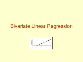
2. Bivariate linear regression • Causality (from x to y) is assumed • The error termembodies anything which is not accounted for by the linear relationship • The unknown parameters(a and b) need to be estimated (usually on sample data). We refer to the sample parameter estimates as aand b (Random) error term Dependent variable Intercept Explanatory variable Regression coefficient

3. To study in detail:Least squares estimation of the unknown parameters • For a given value of the parameters, the error (residual) term for each observation is • The least squares parameter estimates are those who minimize the sum of squared errors:

4. To study in detail:Assumptions on the error term • The error term has a zero mean • The variance of the error term does not vary across cases (homoskedasticity) • The error term for each case is independent of the error term for other cases • The error term is also independent of the values of the explanatory (independent) variable • The error term is normally distributed

5. Prediction • Once a and b have been estimated, it is possible to predict the value of the dependent variable for any given value of the explanatory variable Example: change in price x, what happens in consumption y?

6. Model evaluation • An evaluation of the model performance can be based on the residuals ( ), which provide information on the capability of the model predictions to fit the original data (goodness-of-fit) • Since the parameters a and b are estimated on the sample, just like a mean, they are accompanied by the standard error of the parameters, which measures the precision of these estimates and depends on the sampling size. • Knowledge of the standard errors opens the way to run hypothesis testing.

7. Hypothesis testing on regression coefficients • T-test on each of the individual coefficients • Null hypothesis: the corresponding population coefficient is zero. • The p-value allows one to decide whether to reject or not the null hypothesis that coeff.=zero, (usually p<0.05 reject the null hyp.) • F-test (multiple independent variables, as discussed later) • It is run jointly on all coefficients of the regression model • Null hypothesis: all coefficients are zero • The F-test in linear regression corresponds to the ANOVA test

8. COEFFICIENT OF DETERMINATION R2 The natural candidate for measuring how well the model fits the data is the coefficient of determination, which varies between zero (when the model does not explain any of the variability of the dependent variable) and 1 (when the model fits the data perfectly) Definition: A statistical measure of the ‘goodness of fit’ in a regression equation. It gives the proportion of the total variance of the forecasted variable that is explained by the fitted regression equation, i.e. the independent explanatory variables. 8

9. Bivariate regression in SPSS

10. Regression output Only 5% of total variation is explained by the model (correlation is 0.23) The F-test rejects the hypothesis that all coefficients are zero Both parameters are statistically different from zero according to thet-test

11. MULTIPLE REGRESSION The principle is identical to bivariate regression, but there are more explanatory variables

12. Additional issues: Collinearity (or multicollinearity) problem: • The independent variables must be also independent of each other. • Otherwise we could run into some double-counting problem and it would become very difficult to separate the meaning. • Inefficient estimates • Apparently good model but poor forecasts

13. Goodness-of-fit • The coefficient of determination R2 always increases with the inclusion of additional regressors • Thus, a proper indicator is the adjusted R2which accounts for the number of explanatory variables (k) in relation to the number of observations (n)

14. Multiple regression in SPSS Analyze / Regression / Linear Simply select more than one explanatory variable

15. Output The model accounts for 19.3% of variability in the dependent variable. After adjusting for the number of regressors, the R2 is 0.176 The null hypothesis that all regressors are zero is strongly rejected

16. Output Only these parameters (price, “we like..” and household size) emerge as significantly different from 0. 16

17. Coefficient interpretation – intercept • The constant represents the amount spent being zero all other variables. It provides a negative value, but the hypothesis that the constant is zero is not rejected • A household of zero components, with no income is unlikely to consume chicken • However, estimates for the intercept are often unsatisfactory, because frequently there are no data points with values for the independent variables close or equal to zero

18. Coefficient interpretation • The significant coefficients tell one that: • Each additional household component means an increase in consumption by 277 grams • A £ 1 increase in price leads to a decrease in consumption by 109 grams.