Download
1 / 14
140 likes | 331 Views
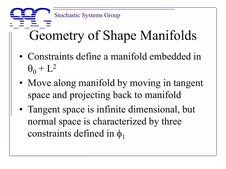
Geometry of Shape Manifolds. Constraints define a manifold embedded in q 0 + L 2 Move along manifold by moving in tangent space and projecting back to manifold Tangent space is infinite dimensional, but normal space is characterized by three constraints defined in f 1. Tangents and Normals.

E N D
Geometry of Shape Manifolds • Constraints define a manifold embedded in q0 + L2 • Move along manifold by moving in tangent space and projecting back to manifold • Tangent space is infinite dimensional, but normal space is characterized by three constraints defined in f1
Tangents and Normals • The derivative of f1 in the direction of f at is: • Implies df1 is surjective • If f is orthogonal to {1, sin q, cos q}, then df1=0 in the direction of f and hence f is in the tangent space
Projections • Want to find the closest element in C1 to an arbitrary qq0 + L2 • Basic idea: move orthogonal to level sets so projections under f form a straight line in R3 • For a point b R3, we define the level set as: • Let b1=(p,0,0). Then its level set is the preshape space C1
Approximate Projections • If points are close to C1, then one can use a faster method • Let dq be the normal vector at q for which f(q+dq)=b1. Can do first order approximation to compute this • Approximate Jacobian as:
Iterative algorithm • Define the residual (error) vector as • Then: where • Iteratively update q + dqq until the error goes to zero • Call this projection operator P
Example Projections Fig. 1: Projections of arbitrary curves into C1
Geodesics • Definition: For a manifold embedded in Euclidean space, a geodesic is a constant speed curve whose acceleration vector is always perpendicular to the manifold • Define the metric between two shapes as the distance along the manifold between the shapes with respect to the L2 inner product • Nice features: • Defined for all closed curves • Interpolants are closed curves • Finds geodesics in a local sense, not necessarily global
Paths from initial conditions • Assume we have a q in C1 and an f in the tangent space • Approximate geodesic along manifold by moving to q+fDt and projecting that back onto the manifold (Dt is step size) • So q(t+Dt) = P(q(t)+f(t)Dt)
Transporting the tangent vector • Now f(t) is not in the tangent space of q(t+Dt) • Two conditions for a geodesic: • The acceleration vector must be perpendicular to the manifold: simply project f into the next tangent space • The curve must move at constant speed: renormalize so ||f(t+1)||=||f(t)|| • hk is the orthonormal basis of the normal space
Geodesics on shape spaces • S1 is a quotient space of C1 under actions of S1 by isometries, so finding geodesics in S1 equivalent to finding geodesics in C1 which are orthogonal to S1 orbits • S1 acting by isometries implies that if a geodesic in preshape space is orthogonal to one S1 orbit, it’s orthogonal to all S1 orbits which it meets • So now normal space has one additional component spanned by • The algorithm is the same as detailed earlier except with an expanded normal space
Geodesics between shapes • We know how to generate geodesic paths given q and f • Now we want to construct a geodesic path from q1 to q2 • So we need to find all f that lead from q1 to an S1 orbit of q2 in unit time, and then choose the one that leads to the shortest path • Let Y define the geodesic flow, with (q1,0,f)=q1 as the initial condition • We then want Y(q1,1,f)=q2
Finding the geodesic • Define an error functional which measures how close we are to the target at t=1: • Choose the geodesic as the flow Y which has the smallest initial velocity ||f|| • i.e., min ||f|| s.t. H[f]=0 • Hard because infinite dimensional search
Fourier decomposition • f L2, so it has a Fourier decomposition • Approximate f with its first m+1 cosine components and its first m sine components: • Let a be the vector containing all of the Fourier coefficients • Now optimization problem is min ||a|| s.t. H[a]=0
Geodesic paths Fig. 2: Geodesic paths between two shapes