Download
1 / 23
240 likes | 271 Views
This comprehensive guide explores spatial econometric analysis, covering spatial data, dependence, heterogeneity, and more. Learn about least squares estimator, nonparametric treatment, autocorrelation, and spatial weighting matrices. Discover spatial lag variables, models, examples, and references in GAUSS.

E N D
Spatial Econometric AnalysisUsing GAUSS 1 Kuan-Pin LinPortland State University
Introduction to Spatial Econometric Analysis • Spatial Data • Cross Section • Panel Data • Spatial Dependence • Spatial Heterogeneity • Spatial Autocorrelation
Spatial Dependence • Least Squares Estimator
Spatial DependenceNonparametric Treatment • Robust Inference • Spatial Heteroscedasticity Autocorrelation Variance-Covariance Matrix
Spatial DependenceNonparametric Treatment • SHAC Estimator • Kernel Function • Normalized Distance
Spatial DependenceParametric Representation • Spatial Weights Matrix • Spatial Contiguity • Geographical Distance • First Law of Geography: Everything is related to everything else, but near things are more related than distant things. • K-Nearest Neighbors
Spatial DependenceParametric Representation • Characteristics of Spatial Weights Matrix • Sparseness • Weights Distribution • Eigenvalues • Higher-Order of Spatial Weights Matrix • W2, W3, … • Redundandency • Circularity
Spatial Weights MatrixAn Example • 3x3 Rook Contiguity • List of 9 Observations with 1-st Order Contiguity, #NZ=24
Spatial Lag Variables • Spatial Independent Variables • Spatial Dependent Variables • Spatial Error Variables
Spatial Econometric Models • Linear Regression Model with Spatial Variables • Spatial Lag Model • Spatial Mixed Model • Spatial Error Model
Examples • Anselin (1988): Crime Equation • Basic Model(Crime Rate) = a + b (Family Income) + g (Housing Value) + e • Spatial Lag Model(Crime Rate) = a + b (Family Income) + g (Housing Value) + l W (Crime Rate) + e • Spatial Error Model(Crime Rate) = a + b (Family Income) + g (Housing Value) + ee = r We + u • Data (anselin.txt, anselin_w.txt)
Examples • China Provincial GDP Output Function • Basic Modelln(GDP) = a + b ln(L) + g ln(K) + e • Spatial Mixed Model ln(GDP) = a + b ln(L) + g ln(K) + bw W ln(L) + gw W ln(K) + l W ln(GDP) + e • Data (china_gdp.txt, china_l.txt, china_k.txt, china_w.txt)
Examples • Ertur and Kosh (2007): International Technological Interdependence and Spatial Externalities • 91 countries, growth convergence in 36 years (1960-1995) • Spatial Lag Solow Growth Modelln(y(t)) - ln(y(0)) = a + b ln(y(0)) + g ln(s) + g ln(n+g+d) + l W ln(y(t)) - ln(y(0))) + e • Data (data-ek.txt)
References • L. Anselin, Spatial Econometrics: Methods and Models. Kluwer Academic Publishers, Boston, 1988. • L. Anselin. “Spatial Econometrics,” In T.C. Mills and K. Patterson (Eds.), Palgrave Handbook ofEconometrics: Volume 1, Econometric Theory. Basingstoke, Palgrave Macmillan, 2006: 901-969. • L. Anselin, “Under the Hood: Issues in the Specification and Interpretation of Spatial Regression Models,” Agricultural Economics 17 (3), 2002: 247-267. • T.G. Conley, “Spatial Econometrics” Entry for New Palgrave Dictionary of Economics, 2nd Edition, S Durlauf and L Blume, eds. (May 2008). • C. Ertur and W. Kosh, “Growth, Technological Interdependence, Spatial Externalities: Theory and Evidence,” Journal of Econometrics, 2007. • J. LeSage and R.K. Pace, Introduction to Spatial Econometrics, Chapman & Hall, CRC Press, 2009. • H. Kelejian and I.R. Prucha, “HAC Estimation in a Spatial Framework,” Journal of Econometrics, 140: 131-154.