Download
1 / 45
450 likes | 483 Views
Explore the advantages of parametric forms, Hermite curves, Bézier curves, algebraic representations, and their properties in computer graphics. Discover the matrix forms and practical applications offered by these curve types.

E N D
Parametric Representations • 3 basic representation strategies: • Explicit: y = mx + b • Implicit: ax + by + c = 0 • Parametric: P = P0 + t (P1 - P0) • Advantages of parametric forms • More degrees of freedom • Directly transformable • Dimension independent • No infinite slope problems • Separates dependent and independent variables • Inherently bounded • Easy to express in vector and matrix form • Common form for many curves and surfaces University of Texas at Austin CS384G - Computer Graphics Fall 2008 Don Fussell 2
Algebraic Representation • All of these curves are just parametric algebraic polynomials expressed in different bases • Parametric linear curve (in E3) • Parametric cubic curve (in E3) • Basis (monomial or power) University of Texas at Austin CS384G - Computer Graphics Fall 2008 Don Fussell 3
Hermite Curves • 12 degrees of freedom (4 3-d vector constraints) • Specify endpoints and tangent vectors at endpoints • Solving for the coefficients: pu(1) pu(0) • p(1) u = 1 • u = 0 p(0) University of Texas at Austin CS384G - Computer Graphics Fall 2008 Don Fussell 4
Hermite Curves - Hermite Basis • Substituting for the coefficients and collecting terms gives • Call the Hermite blending functions or basis functions • Then H2 H1 H3 n H4 University of Texas at Austin CS384G - Computer Graphics Fall 2008 Don Fussell 5
Hermite Curves - Matrix Form • Putting this in matrix form • MH is called the Hermite characteristic matrix • Collecting the Hermite geometric coefficients into a geometry vector B, we have a matrix formulation for the Hermite curve p(u) University of Texas at Austin CS384G - Computer Graphics Fall 2008 Don Fussell 6
Hermite and Algebraic Forms • MH transforms geometric coefficients (“coordinates”) from the Hermite basis to the algebraic coefficients of the monomial basis University of Texas at Austin CS384G - Computer Graphics Fall 2008 Don Fussell 7
p2 p3 • k1 p(u) k2 p1 p0 Cubic Bézier Curves • Specifying tangent vectors at endpoints isn’t always convenient for geometric modeling • We may prefer making all the geometric coefficients points, let’s call them control points, and label them p0, p1, p2, and p3 • For cubic curves, we can proceed by letting the tangents at the endpoints for the Hermite curve be defined by a vector between a pair of control points, so that: University of Texas at Austin CS384G - Computer Graphics Fall 2008 Don Fussell 8
Cubic Bézier Curves • Substituting this into the Hermite curve expression and rearranging, we get • In matrix form, this is University of Texas at Austin CS384G - Computer Graphics Fall 2008 Don Fussell 9
Cubic Bézier Curves • What values should we choose for k1 and k2? • If we let the control points be evenly spaced in parameter space, then p0 is at u = 0, p1 at u = 1/3, p2 at u = 2/3 and p3 at u = 1. Then and k1 = k2 = 3, giving a nice symmetric characteristic matrix: • So University of Texas at Austin CS384G - Computer Graphics Fall 2008 Don Fussell 10
General Bézier Curves • This can be rewritten as • Note that the binomial expansion of (u + (1 - u))n is • This suggests a general formula for Bézier curves of arbitrary degree University of Texas at Austin CS384G - Computer Graphics Fall 2008 Don Fussell 11
General Bézier Curves • The binomial expansion gives the Bernstein basis (or Bézier blending functions)Bi,nfor arbitrary degree Bézier curves • Of particular interest to us (in addition to cubic curves): • Linear: p(u) = (1 - u)p0 + up1 • Quadratic: p(u) = (1 - u)2p0 + 2u(1 - u)p1 + u2p2 B0,3 B3,3 Cubic Bézier Blending Functions B1,3 B2,3 n University of Texas at Austin CS384G - Computer Graphics Fall 2008 Don Fussell 12
p3 p1 p0 p2 Bézier Curve Properties • Interpolates end control points, not middle ones • Stays inside convex hull of control points • Important for many algorithms • Because it’s a convex combination of points, i.e. affine with positive weights • Variation diminishing • Doesn’t “wiggle” more than control polygon University of Texas at Austin CS384G - Computer Graphics Fall 2008 Don Fussell 13
Rendering Bézier Curves • We can obtain a point on a Bézier curve by just evaluating the function for a given value of u • Fastest way, precompute A=MBP once control points are known, then evaluate p(ui)=[ui3ui2ui 1]A, i = 0,1,2,…,n for n fixed increments of u • For better numerical stability, take e.g. a quadratic curve (for simplicity) and rewrite • This is just a linear interpolation of two points, each of which was obtained by interpolating a pair of adjacent control points University of Texas at Austin CS384G - Computer Graphics Fall 2008 Don Fussell 14
de Casteljau Algorithm • This hierarchical linear interpolation works for general Bézier curves, as given by the following recurrence where pi,0 i = 0,1,2,…,n are the control points for a degree n Bézier curve and p0,n = p(u) • For efficiency this should not be implemented recursively. • Useful for point evaluation in a recursive subdivision algorithm to render a curve since it generates the control points for the subdivided curves. University of Texas at Austin CS384G - Computer Graphics Fall 2008 Don Fussell 15
de Casteljau Algorithm Starting with the control points and a given value of u In this example, u≈0.25 p1 p0 p2 p3 University of Texas at Austin CS384G - Computer Graphics Fall 2008 Don Fussell 16
de Casteljau Algorithm p1 q1 q0 p0 p2 q2 p3 University of Texas at Austin CS384G - Computer Graphics Fall 2008 Don Fussell 17
de Casteljau Algorithm q1 r0 q0 r1 q2 University of Texas at Austin CS384G - Computer Graphics Fall 2008 Don Fussell 18
de Casteljau Algorithm r0 • p(u) r1 University of Texas at Austin CS384G - Computer Graphics Fall 2008 Don Fussell 19
p1 • p(u) p0 p2 p3 de Casteljau algorihm University of Texas at Austin CS384G - Computer Graphics Fall 2008 Don Fussell 20
Drawing Bézier Curves • How can you draw a curve? • Generally no low-level support for drawing curves • Can only draw line segments or individual pixels • Approximate the curve as a series of line segments • Analogous to tessellation of a surface • Methods: • Sample uniformly • Sample adaptively • Recursive Subdivision University of Texas at Austin CS384G - Computer Graphics Fall 2008 Don Fussell 21
p(u) p4 p2 p1 p3 p0 Uniform Sampling • Approximate curve with n line segments • n chosen in advance • Evaluate • For an arbitrary cubic curve • Connect the points with lines • Too few points? • Bad approximation • “Curve” is faceted • Too many points? • Slow to draw too many line segments • Segments may draw on top of each other University of Texas at Austin CS384G - Computer Graphics Fall 2008 Don Fussell 22
p(u) Adaptive Sampling • Use only as many line segments as you need • Fewer segments needed where curve is mostly flat • More segments needed where curve bends • No need to track bends that are smaller than a pixel • Various schemes for sampling,checking results, deciding whetherto sample more • Or, use knowledge of curve structure: • Adapt by recursive subdivision University of Texas at Austin CS384G - Computer Graphics Fall 2008 Don Fussell 23
Recursive Subdivision • Any cubic curve segment can be expressed as a Bézier curve • Any piece of a cubic curve is itself a cubic curve • Therefore: • Any Bézier curve can be broken up into smaller Bézier curves • But how…? University of Texas at Austin CS384G - Computer Graphics Fall 2008 Don Fussell 24
de Casteljau subdivision de Casteljau construction points are the control points of two Bézier sub-segments p1 r0 q0 r1 x p0 p2 q2 p3 University of Texas at Austin CS384G - Computer Graphics Fall 2008 Don Fussell 25
Adaptive subdivision algorithm • Use de Casteljau construction to split Bézier segment • Examine each half: • If flat enough: draw line segment • Else: recurse • To test if curve is flat enough • Only need to test if hull is flat enough • Curve is guaranteed to lie within the hull • e.g., test how far the handles are from a straight segment • If it’s about a pixel, the hull is flat University of Texas at Austin CS384G - Computer Graphics Fall 2008 Don Fussell 26
Composite Curves • Hermite and Bézier curves generalize line segments to higher degree polynomials. But what if we want more complicated curves than we can get with a single one of these? Then we need to build composite curves, like polylines but curved. • Continuity conditions for composite curves • C0 - The curve is continuous, i.e. the endpoints of consecutive curve segments coincide • C1 - The tangent (derivative with respect to the parameter) is continuous, i.e. the tangents match at the common endpoint of consecutive curve segments • C2 - The second parametric derivative is continuous, i.e. matches at common endpoints • G0 - Same as C0 • G1 - Derivatives wrt the coordinates are continuous. Weaker than C1, the tangents should point in the same direction, but lengths can differ. • G2 - Second derivatives wrt the coordinates are continuous • … University of Texas at Austin CS384G - Computer Graphics Fall 2008 Don Fussell 27
Composite Bézier Curves • C0, G0 - Coincident end control points • C1 - p3 - p2 on first curve equals p1 - p0 on second • G1 - p3 - p2 on first curve proportional to p1 - p0 on second • C2, G2 - More complex, use B-splines to automatically control continuity across curve segments University of Texas at Austin CS384G - Computer Graphics Fall 2008 Don Fussell 28
u 1 0 knot knot Polar form for Bézier Curves • A much more useful point labeling scheme • Start with knots, “interesting” values in parameter space • For Bézier curves, parameter space is normally [0, 1], and the knots are at 0 and 1. • Now build a knot vector, a non-decreasing sequence of knot values. • For a degree n Bézier curve, the knot vector will have n 0’s followed by n 1’s [0,0,…,0,1,1,…,1] • Cubic Bézier knot vector [0,0,0,1,1,1] • Quadratic Bézier knot vector [0,0,1,1] • Polar labels for consecutive control points are sequences of n knots from the vector, incrementing the starting point by 1 each time • Cubic Bézier control points: p0 = p(0,0,0), p1 = p(0,0,1), p2 = p(0,1,1), p3 = p(1,1,1) • Quadratic Bézier control points: p0 = p(0,0), p1 = p(0,1), p2 = p(1,1) University of Texas at Austin CS384G - Computer Graphics Fall 2008 Don Fussell 29
Polar form rules • Polar values are symmetric in their arguments, i.e. all permutations of a polar label are equivalent. p(0,0,1) = p(0,1,0) = p(1,0,0), etc. • Given p(u1, u2,…,un-1, a) and p(u1, u2,…,un-1, b), for any value c we can compute That is, p(u1, u2,…,un-1, c) is an affine combination of p(u1, u2,…,un-1, a) and p(u1, u2,…,un-1, b) . Examples: University of Texas at Austin CS384G - Computer Graphics Fall 2008 Don Fussell 30
de Casteljau in polar form p(0,0,1) p(0,0,0) p(0,1,1) p(1,1,1) University of Texas at Austin CS384G - Computer Graphics Fall 2008 Don Fussell 31
de Casteljau in polar form p(0,0,1) p(0,u,1) p(0,0,u) p(0,0,0) p(0,1,1) p(u,1,1) p(1,1,1) University of Texas at Austin CS384G - Computer Graphics Fall 2008 Don Fussell 32
de Casteljau in polar form p(0,0,1) p(0,u,1) p(0,u,u) p(0,0,u) p(u,u,1) p(0,0,0) p(0,1,1) p(u,1,1) p(1,1,1) University of Texas at Austin CS384G - Computer Graphics Fall 2008 Don Fussell 33
de Casteljau in polar form p(0,0,1) p(0,u,1) p(0,u,u) p(0,0,u) • p(u,u,1) p(u,u,u) p(0,0,0) p(0,1,1) p(u,1,1) p(1,1,1) University of Texas at Austin CS384G - Computer Graphics Fall 2008 Don Fussell 34
de Casteljau in polar form p(0,0,1) p(0,u,1) p(0,u,u) p(0,0,u) • p(u,u,1) p(u,u,u) p(0,0,0) p(0,1,1) p(u,1,1) p(1,1,1) University of Texas at Austin CS384G - Computer Graphics Fall 2008 Don Fussell 35
u 1 0 u 2 knot knot knot Composite curves in polar form • Suppose we want to glue two cubic Bézier curves together in a way that automatically guarantees C2 continuity everywhere. We can do this easily in polar form. • Start with parameter space for the pair of curves • 1st curve [0,1], 2nd curve (1,2] • Make a knot vector: [000,1,222] • Number control points as before: p(0,0,0), p(0,0,1), p(0,1,2), p(1,2,2), p(2,2,2) • Okay, 5 control points for the two curves, so 3 of them must be shared since each curve needs 4. That’s what having only 1 copy of knot 1 achieves, and that’s what gives us C2 continuity at the join point at u = 1 University of Texas at Austin CS384G - Computer Graphics Fall 2008 Don Fussell 36
p(0,0,1) p(0,1,2) p(0,0,0) p(2,2,2) p(1,2,2) de Boor algorithm in polar form u = 0.5 Knot vector = [0,0,0,1,2,2,2] University of Texas at Austin CS384G - Computer Graphics Fall 2008 Don Fussell 37
Inserting a knot p(0,0,1) p(0,0.5,1) p(0,1,2) p(0,0,0.5) p(0.5,1,2) p(0,0,0) p(2,2,2) p(1,2,2) u = 0.5 Knot vector = [0,0,0,0.5,1,2,2,2] University of Texas at Austin CS384G - Computer Graphics Fall 2008 Don Fussell 38
Inserting a 2nd knot p(0,0,1) p(0,0.5,1) p(0.5,0.5,1) p(0,1,2) p(0,0.5,0.5) p(0,0,0.5) p(0.5,1,2) p(0,0,0) p(2,2,2) p(1,2,2) u = 0.5 Knot vector = [0,0,0,0.5,0.5,1,2,2,2] University of Texas at Austin CS384G - Computer Graphics Fall 2008 Don Fussell 39
Inserting a 3rd knot to get a point p(0,0,1) p(0,0.5,1) p(0.5,0.5,1) p(0,1,2) p(0,0.5,0.5) p(0.5,0.5,0.5) p(0,0,0.5) p(0.5,1,2) p(0,0,0) p(2,2,2) p(1,2,2) u = 0.5 Knot vector = [0,0,0,0.5,0.5,0.5,1,2,2,2] University of Texas at Austin CS384G - Computer Graphics Fall 2008 Don Fussell 40
Recovering the Bézier curves p(0,0,1) p(0,1,1) p(0,1,2) p(1,1,2) p(0,0,0) p(2,2,2) p(1,2,2) Knot vector = [0,0,0,1,1,2,2,2] University of Texas at Austin CS384G - Computer Graphics Fall 2008 Don Fussell 41
Recovering the Bézier curves p(0,0,1) p(0,1,1) p(0,1,2) p(1,1,1) p(1,1,2) p(0,0,0) p(2,2,2) p(1,2,2) Knot vector = [0,0,0,1,1,1,2,2,2] University of Texas at Austin CS384G - Computer Graphics Fall 2008 Don Fussell 42
B-Splines • B-splines are a generalization of Bézier curves that allows grouping them together with continuity across the joints • The B in B-splines stands for basis, they are based on a very general class of spline basis functions • Splines is a term referring to composite parametric curves with guaranteed continuity • The general form is similar to that of Bézier curves Given m + 1 values ui in parameter space (these are called knots), a degree n B-spline curve is given by: where m i + n + 1 University of Texas at Austin CS384G - Computer Graphics Fall 2008 Don Fussell 43
Uniform periodic basis • Let N(u) be a global basis function for our uniform cubic B-splines • N(u) is piecewise cubic p(u) = N(u) p3+ N(u+1) p2 + N(u+2) p1 + N(u+3)p0 N(u) u 4 0 2 1 3 p3 p2 p1 p0 University of Texas at Austin CS384G - Computer Graphics Fall 2008 Don Fussell 44
Uniform periodic B-Spline p1 p2 p0 p3 p(u) = (–1/6u3 + 1/2u2 – 1/2u + 1/6)p0 + ( 1/2u3– u2 + 2/3)p1 + (–1/2u3 + 1/2u2+ 1/2u + 1/6)p2 + ( 1/6u3 )p3 University of Texas at Austin CS384G - Computer Graphics Fall 2008 Don Fussell 45