Download
1 / 30
300 likes | 329 Views
The t Tests. Independent Samples. The t Test for Independent Samples. Observations in each sample are independent (not from the same population) each other. We want to compare differences between sample means. Sampling Distribution of the Difference Between Means.

E N D
The t Tests Independent Samples
The t Test for Independent Samples • Observations in each sample are independent (not from the same population) each other. • We want to compare differences between sample means.
Sampling Distribution of the Difference Between Means • Imagine gathering two samples from the same population. • And then subtracting the mean of one from the mean of the other… • If you create a sampling distribution of the difference between the means… • Given the null hypothesis, we expect the mean of the sampling distribution of differences, 1- 2, to be 0. • We must estimate the standard deviation of the sampling distribution of the difference between means (i.e., the standard error of the difference between means).
Pooled Estimate of the Population Variance • Using the assumption of homogeneity of variance, both s1 and s2 are estimates of the same population variance. • If this is so, rather than make two separate estimates, each based on some small sample, it is preferable to combine the information from both samples and make a single pooled estimate of the population variance.
Pooled Estimate of the Population Variance • The pooled estimate of the population variance becomes the average of both sample variances, once adjusted for their degrees of freedom. • Multiplying each sample variance by its degrees of freedom ensures that the contribution of each sample variance is proportionate to its degrees of freedom. • You know you have made a mistake in calculating the pooled estimate of the variance if it does not come out between the two estimates. • You have also made a mistake if it does not come out closer to the estimate from the larger sample. • The degrees of freedom for the pooled estimate of the variance equals the sum of the two sample sizes minus two, or (n1-1) +(n2-1).
The t Test for Independent Samples: An Example • Stereotype Threat “This test is a measure of your academic ability.” “Trying to develop the test itself.”
The t Test for Independent Samples: An Example • State the research question. • Does stereotype threat hinder the performance of those individuals to which it is applied? • State the statistical hypotheses.
The t Test for Independent Samples: An Example • Set the decision rule.
The t Test for Independent Samples: An Example • Calculate the test statistic.
The t Test for Independent Samples: An Example • Calculate the test statistic.
The t Test for Independent Samples: An Example • Calculate the test statistic.
The t Test for Independent Samples: An Example • Decide if your result is significant. • Reject H0, - 2.37< - 1.721 • Interpret your results. • Stereotype threat significantly reduced performance of those to whom it was applied.
Assumptions 1) The observations within each sample must be independent. 2) The two populations from which the samples are selected must be normal. 3) The two populations from which the samples are selected must have equal variances. • This is also known as homogeneity of variance, and there are two methods for testing that we have equal variances: • a) informal method – simply compare sample variances • b) Levene’s test – We’ll see this on the SPSS output • Random Assignment To make causal claims • Random Sampling To make generalizations to the target population
Effect Size 1) Simply report the actual results of the study. • (a) Most direct method. • (b) Can be misleading. 2) Calculate Cohen’s d or Δ (preferred). (a) Magnitude of effect size is standardized by measuring the mean difference between two treatments in terms of the standard deviation. (b) d = (M1-M2)/sp2 (c) Evaluate using the following criteria: • i) .20 small effect • ii) .50 medium effect • iii) > .80 large effect
Effect Size: Example • In the study evaluating stereotype threat, the null hypothesis was rejected, with M1=6.58, M2=9.64, and sp2 = 9.59. • Calculate Cohen’s d, and evaluate the magnitude of this measure (small, medium, or large). • Compare effect size to z table to determine where the mean of one group is relative to the other.
Type 1 Error & Type 2 Error Scientist’s Decision Reject null hypothesis Fail to reject null hypothesis Type 1 Error Correct Decision probability = Probability = 1- Correct decision Type 2 Error probability = 1 - probability = Null hypothesis is true Null hypothesis is false Type 1 Error = Type 2 Error = Cases in which you reject null hypothesis when it is really true Cases in which you fail to reject null hypothesis when it is false
Power and sample size estimation • Power is the probability of correctly rejecting a null hypothesis. • In social sciences we typically use .80. • What determines the power of a study • Effect size • Sample size • Variance • α • One vs. two tailed tests
If you want to know • Sample Size • Need to know • α • β • Δ • Power • Need to know • α • N per condition • Δ
Calculating sample size • Remember stereotype threat example • Δ = .99 • Say we want to perform a test with • power (1-β) = .80 • Two tailed alpha = .05
Calculating power • Say we did the same study with n of 5 in each condition (N =10) • We want to know how much power we have to find d or Δ= .99. • Again we are using a two tailed test with α = .05.
Spss: Homework Hint • For the two sample t tests you will need to create two variables, cond (X) and score (Y)