Experiments with Random Factors

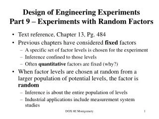
1. Experiments with Random Factors • Previous chapters have considered fixed factors • A specific set of factor levels is chosen for the experiment • Inference confined to those levels • Often quantitative factors are fixed (why?) • When factor levels are chosen at random from a larger population of potential levels, the factor is random • Inference is about the entire population of levels • Industrial applications include measurement system studies

2. Random Effects Models • In the fixed effects models, the main interest is the treatment means • In random effects models, the knowledge about the particular ones investigated is relatively useless, but the variability is the primary concern • The population of factor levels is of infinite size, or is large enough to be considered infinite

3. Random Effects Models • The usual single factor ANOVA model is • Now both the error term and the treatment effects are random variables: • Variancecomponents: • Total variability in the observations is partitioned into • 1. A component that measures the variability between the treatments, and • 2. A component that measures the variability within treatments • The sums of squares SST = SSTreatment + SSE

4. Relevant Hypotheses in the Random Effects (or Components of Variance) Model • In the fixed effects model we test equality of treatment means • This is no longer appropriate because the treatments are randomly selected • the individual ones we happen to have are not of specific interest • we are interested in the population of treatments • The appropriate hypotheses are

5. Testing Hypotheses - Random Effects Model • The standard ANOVA partition of the total sum of squares still works; leads to usual ANOVA display • Form of the hypothesis test depends on the expectedmeansquares and • Therefore, the appropriate test statistic is • Ho is rejected if Fo > Fa,a-1,N-a

6. Estimating the Variance Components • Use the ANOVA method; equate expected mean squares to their observed values: • Potential problems with these estimators • Negative estimates (woops!) • They are moment estimators & don’t have best statistical properties

7. Random Effects Models • Example 13-1 (pg. 467) – weaving fabric on looms • Response variable is strength • Interest focuses on determining if there is difference in strength due to the different looms • However, the weave room contains many (100s) looms • Solution – select a (random) sample of the looms, obtain fabric from each • Consequently, “looms” is a randomfactor

8. It looks like a standard single-factor experiment with a = 4 & n = 4 Table 13-1 Strength Data for Example 13-1

9. Minitab Solution (Balanced ANOVA) Factor Type Levels Values Loom random 4 1 2 3 4 Analysis of Variance for y Source DF SS MS F P Loom 3 89.188 29.729 15.68 0.000 Error 12 22.750 1.896 Total 15 111.938 Source Variance Error Expected Mean Square for Each Term component term (using unrestricted model) 1 Loom 6.958 2 (2) + 4(1) 2 Error 1.896 (2)

10. Random Effects Models • Important use of variance components – isolating of different sources of variability that affect a product or system Figure 13-1

11. Confidence Intervals on the Variance Components • Easy to find a 100(1-)% CI on • Other confidence interval results are given in the book • Sometimes the procedures are not simple

12. Extension to Factorial Treatment Structure • Two factors, factorial experiment, both factors random (Section 13-2, pg. 490) • The model parameters are NID random variables • Random effects model

13. Testing Hypotheses - Random Effects Model • Once again, the standard ANOVA partition is appropriate • The sums of squares are calculated as in the fixed effects case • Relevant hypotheses: • Form of the test statistics depend on the expectedmeansquares:

14. Estimating the Variance Components – Two Factor Random model • As before, use the ANOVA method; equate expected mean squares to their observed values: • Potential problems with these estimators

15. Example 13-2 (pg. 492) A Measurement Systems Capability Study • Gauge capability (or R&R) is of interest • The gauge is used by an operator to measure a critical dimension on a part • Repeatability is a measure of the variability due only to the gauge • Reproducibility is a measure of the variability due to the operator • This is a two-factor factorial (completely randomized) with both factors (operators, parts) random – a random effects model

16. Table 13-3 13-2

17. Example 13-2 • The objective is estimating the variance components • is gauge repeatability • is reproducibility of the gauge • The variance components:

18. Example 13-2 (pg. 494) Minitab Solution – Using Balanced ANOVA Source DF SS MS F P Part 19 1185.425 62.391 87.65 0.000 Operator 2 2.617 1.308 1.84 0.173 Part*Operator 38 27.050 0.712 0.72 0.861 Error 60 59.500 0.992 Total 119 1274.592 Source Variance Error Expected Mean Square for Each Term component term (using unrestricted model) 1 Part 10.2798 3 (4) + 2(3) + 6(1) 2 Operator 0.0149 3 (4) + 2(3) + 40(2) 3 Part*Operator -0.1399 4 (4) + 2(3) 4 Error 0.9917 (4)

19. Example 13-2 (pg. 494) Minitab Solution – Balanced ANOVA • There is a large effect of parts (not unexpected) • Small operator effect • No Part – Operator interaction • Negative estimate of the Part – Operator interaction variance component • Fit a reduced model with the Part – Operator interaction deleted yijk = m + ti + bj + eijk

20. Example 13-2 (pg. 494) Minitab Solution – Reduced Model Source DF SS MS F P Part 19 1185.425 62.391 70.64 0.000 Operator 2 2.617 1.308 1.48 0.232 Error 98 86.550 0.883 Total 119 1274.592 Source Variance Error Expected Mean Square for Each Term component term (using unrestricted model) 1 Part 10.2513 3 (3) + 6(1) 2 Operator 0.0106 3 (3) + 40(2) 3 Error 0.8832 (3)

21. Example 13-2 (pg. 495) Minitab Solution – Reduced Model • The expected mean squares are • Estimating the variance components • Estimating gauge capability: ?