Download
1 / 22
220 likes | 235 Views
Einstein@Home. Bruce Allen, U. Wisconsin - Milwaukee and AEI. Overview. Status of Einstein@Home Users, credits, size Officially funded as a project by NSF! Status of the “old style” S3 analysis Done and reviewed! Status of the S4 analysis

E N D
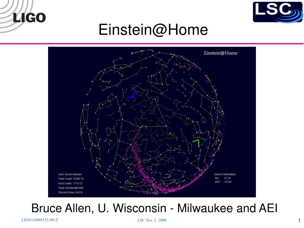
Einstein@Home Bruce Allen, U. Wisconsin - Milwaukee and AEI
Overview • Status of Einstein@Home • Users, credits, size • Officially funded as a project by NSF! • Status of the “old style” S3 analysis • Done and reviewed! • Status of the S4 analysis • Postprocessing underway since mid-summer, still ongoing • First careful estimation of search sensitivity (for practice, not for publication!) • Status of the S5 analysis (16 446 454 workunits x 5 CPU hours x 2) • Processing 49% complete • About 100 more days of processing to go • Einstein@Home server/project up and operational with no glitches for 143 days! • Status of the upcoming hierarchial S5 analysis • First CW analysis that integrates long (> 30 min) coherent and an incoherent methods • Gives us the optimal sensitivity for our CPU power • No large data transfers to or from the host machines.
User/Credit History http://www.boincsynergy.com/stats/
Current performance http://www.boincstats.com/ Einstein@Home is currently getting 84 Tflops
Status of S3 Analysis • Finished: • Final S3 analysis and writeup have been reviewed and approved by the CW Review Committee and the LSC Executive Committee. • Results are posted on the Einstein@Home web site. • We didn’t find any CW sources
Overview of S4 analysis • Coherently analyzed 30-hour data stretches (10 LHO, 7 LLO) 540 hours total. Spanned times vary, but all < 40 hours. • Searched 50 Hz - 1500 Hz in 6,731,410 work units from 24-12-2005 to 20-7-2006. • Near optimal grid (within ~2) on the sky and in frequency and df/dt • Explicit search over spindowns (df/dt) corresponding to pulsars older than a few thousand years. Previous searches had |df/dt|<1/(integration time)2. • Each host searches the entire sky and fdot range and a variable-sized region of frequency df ~ f-3 and one stretch of data. It then returns list of ‘top 13,000 events’. • Range of frequency that decreases with increasing frequency as f^-3 • f<300 Hz: mismatch 0.2, spin-down ages > 1,000 years • f300 Hz: mismatch 0.5, spin-down ages > 10,000 years • Each workunit produces a compressed data file that is about 150kB in size. • The total data volume to post-process is 1 TB (compressed) or 4 TB (uncompressed). Many hardware improvements “behind the scenes” to handle this data volume and permit postprocessing on Nemo cluster.
S4 post-processingcoincidence strategy • Search for signals that appear in each of the 17 different data stretches, with consistent parameters • Steps: • Shift candidate frequencies to a fixed fiducial time • ‘Bin’ candidates in four dimensions (alpha, delta, f, fdot) • Search for bins which have candidates from many of the 17 data stretches • Span entire sky, entire frequency band, entire fdot band. • Bins are chosen to be as small as possible, consistent with: • Sky bin size > largest grid separations (use Gaussian model in delta) • Frequency bin size > frequency resolution + (grid spacing in fdot) x T • Fdot bin size > Fdot grid spacing • Bins are also shifted by 1/2 the bin width in all 2^4 combinations, so as not to miss any candidates on opposite sides of cell faces.
How many events to keep? • Goal: constant false alarm probability per data stretch per coincidence cell. • Why: in the coincidence analysis, this makes it easier to interpret the results and to predict false alarm probability. • How: in a given frequency band, keep the same number of events from each data stretch. • How many events to keep: to get a false alarm probability of 0.1% to find 7 or more coincidences (out of 17) in random noise in a 1/2 Hz band. • Example: band 123.0-123.5 Hz: • Data stretch 1 (10 workunits): keep top 1000 events per workunit • Data stretch 2 (5 workunits): keep top 2000 events per workunit • Data stretch 3 (8 workunits): keep top 1250 events per workunit… • Data stretch 17 (20 workunits): keep top 500 events per workunit
Coincidence Analysis Grids • Typical sky grid has points separated more broadly near the equator. • Each of the 17 data segments has a different grid • In doing the coincidence analysis we use a Gaussian fit to the declination differences to ensure that we don’t miss correlated events.
Sample results (120-130 Hz) • Number of events:54,841 x 17 per 1/2 Hz • Number of coincidence cells per 1/2 Hz: 5,398,250 • Max coincidences found: 5
Sample results (260-270 Hz) • Number of events: 166,033 x 17 per 1/2 Hz • Number of coincidence cells per 1/2 Hz: 19,747,000 • Max coincidences found: 7(Line: “Yousuke’s 8 Hz comb”, onlyin L1)
Sample results (100-110 Hz) • Number of events: 40,364 x 17 per 1/2 Hz • Number of coincidence cells per 1/2 Hz: 5,398,250 • Max coincidences found: 11This is fake pulsar #3. Injection was off for 5 of the 17 data stretches.
Complete S4 results (50-1500 Hz) • More work still needed: • Postprocessing being repeated to fix some mistakes made the first time (wrong counting of coincidence cells led to wrong false alarm rate). • After removal of hardware injections, need to follow up outliers
Determining S4 sensitivity • Holger Pletsch has developed methods to estimate the sensitivity and has tested this using software injections. • For a given signal, did analytic estimate the 2F values in each of the 17 data segments to determine how many times it falls in the top list of candidates. • This method correctly predicts how many coincidences would be observed. • Repeat for 500 randomly placed and oriented simulated signals per 0.5 Hz band • Note: v1 calibration
Current S5 run • Very similar to previous S4 run, but more data(22 x 30 hours) which is also more sensitive • Postprocessing not even started yet • Search has been underway for about 140 days • About 100 days of work left
Next S5 Search • The CW group is planning to start running the first true Einstein@Home hierarchicalsearch in about 3 months! • All-sky, TBD: f < ~900 Hz, spindown ages > 10000 years • A new search code (union of multi-detector Fstat and Hough). A stack-slide incoherent option is also “in the works”. • This will use approximately 96 x 20 hours of coincident H1/L1 data (adding strains to gain factor of sqrt(2) in strain sensitivity) • Combines coherent Fstat method with incoherent Hough method (48 25-hour stacks) • Many CW group members are working very hard on this: Krishnan, Prix, Machenschalk, Siemens, Hammer, Mendell, Sintes, Papa, and others. • Should permit a search that extends hundreds of pc into the Galaxy • This should become the most sensitive blind CW search possible with current knowledge and technology • As soon as we can: a coherent follow-up integration stage.
Next S5 search: data selection Tdata = Nstack Tcoherent and hmin ~ Tcoherent-1/2 Nstack-1/4 • Constraints and tradeoffs • Practical: smaller data Tdata volume is good for Einstein@Home users; larger data volume gives more sensitivity & confidence • Sensitivity: larger Tcoherent gives more sensitivity but less data. Coincident data increases sensitivity by sqrt(2) but yields less data • CPU cost: larger Tcoherent increases cost of coherent stage relative to incoherent Hough stage • Study carried out by Siemens, Prix, and Krishnan • Determine much data would be available as a function of Tcoherent with and without 2-detector coincidence • Extrapolate to January 2007, and estimate • sensitivity hmin • total data volume Tdata • computational cost = sum of the two different search stages
Next S5 search: data selection Tdata Tstack Nstack hmin CPU_inc CPU_coh CPU data_volume 12h 16h 535 1.00 1.00 1.00 1.00 1.00 15h 20h 401 1.04 1.71 2.86 1.72 0.94 20h 25h 226 1.04 1.66 6.56 1.67 0.70 … LHO … LLO Tstack Tdata Tdata Tstack Nstack hmin CPU_inc CPU_coh CPU data_volume 12h 16h 320 1.05 0.09 0.60 0.09 0.60 15h 20h 236 1.08 0.15 1.68 0.15 0.55 20h 25h 96 1.00 0.07 2.79 0.08 0.30 … LHO LLO
Coherent + incoherent “merge” Time Keep 1/5 of peaks (lots of data!) … Detector Frequency FFT FFT FFT Make Hough maps FFT Current Hough analysis Integrated code for Einstein@Home analysis Code 1 Code 2 … Time Keep 1/4 of peaksToo much data tostore or transmit Source Frequency Fstat Fstat Make Hough maps For Einstein@Home, the multi-IFO Fstat (Code 1) and Hough (Code 2) had to be merged into a single stand-alone executable that could pass the needed data between the two stages. This has been done by Krishnan. Also planned: integrate the Stack-Slide incoherent step as an alternative to Hough.
Conclusions • Einstein@Home is healthy and growing, and providing 10x more CPU cycles than other LSC resources. • S4 analysis postprocessing is making good progess. First reliable estimates of the sensitivity. • Similar S5 analysis should be finished in 3 - 6 months. • Ambitions plans to run the first true hierarchical search under Einstein@Home on S5 data in just a few months.