Download
1 / 15
150 likes | 262 Views
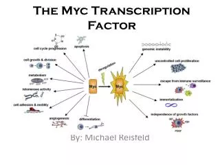
Gaussian Processes for Transcription Factor Protein Inference. Neil D. Lawrence, Guido Sanguinetti and Magnus Rattray. Talk plan. Biological problem Dynamical models of gene expression Introducing GPs in the equation Linear and non-linear response Results Future extensions?. Transcription.

E N D
Gaussian Processes forTranscription Factor Protein Inference Neil D. Lawrence, Guido Sanguinetti and Magnus Rattray
Talk plan • Biological problem • Dynamical models of gene expression • Introducing GPs in the equation • Linear and non-linear response • Results • Future extensions?
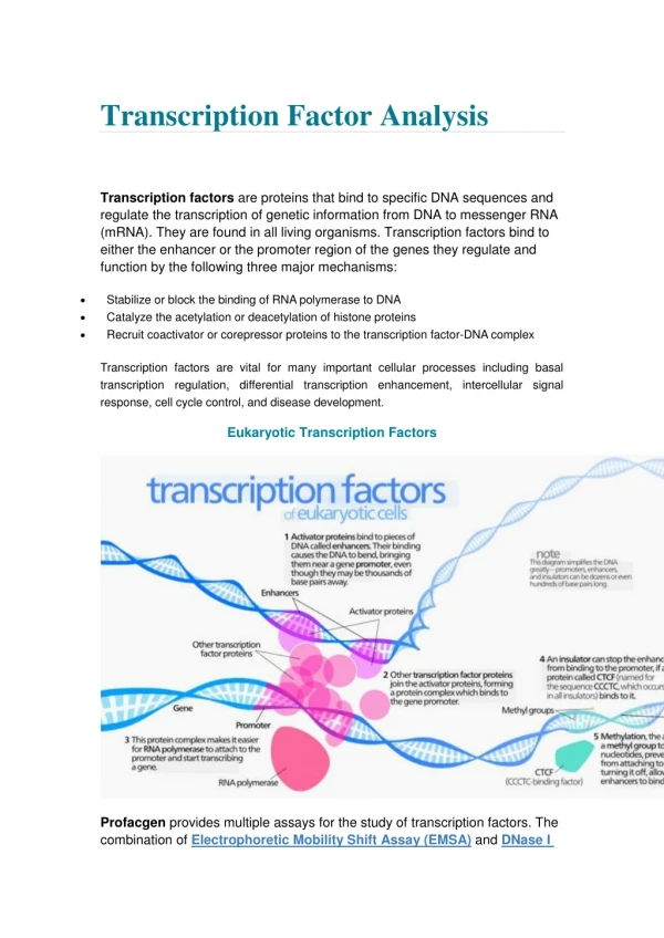
Transcription • Transcription is the process by • which the genetic information • stored in DNA is expressed as • mRNA molecules. • It is promoted or repressed by • proteins known as transcription • Factors (TFs). • TF concentrations are hard to measure. • The effect of TFs on gene expression is hard to quantify precisely. From Alberts et al., Molecular Biology of the Cell
Simplified model • Consider only one transcription factor binding some target genes TF ...... g1 g2 gN Model in detail this simplified situation, turning hard experimental problems into inference tasks.
Modelling transcription • Quantitative description of transcriptional regulation can be achieved only by inference. • Assume a simplified situation where one TF regulates a few targets. Let xj(t) be the mRNA concentration of gene j at time t. Then at equilibrium Here Bj is the baseline expression level, Dj is the decay rate of mRNA for gene j, and f(t) is the TF protein concentration. The function g determines the response of the gene to the TF. Common choices for g are linear (Barenco et al., Gen. Biol.,2006) or Michaelis-Menten (Rogers et al., MASAMB, 2006).
Inference • Bayesian approaches have discretised the system (1) at the observed time points and treated the function values as additional parameters. Estimates of the parameters were obtained by MCMC. • Computationally expensive. • Inference limited to a few points. • Need to evaluate the production rates. This can be difficult as standard techniques (e.g. polynomial interpolation) suffer in the presence of noise.
GPs for Linear response • Treat the system (1) as a continuous system placing a GP prior distribution on f. • Equation (1) can be solved in the linear case As this is a linear operation on the function f, it follows that the mRNA levels are also governed by a GP.
Kernel computations • If we define gi(t)=0tf(u)eDiudu, we get the covariance of gi and gj in terms of the covariance of f as • Wecan then compute the cross covariances between the various mRNA species and the latent function For RBF priors, this can be computed analytically.
We can jointly sample from the (x,f) process. • Parameter estimation can be carried out using type II maximum likelihood. • Posterior distribution for the TF concentrations is obtained by standard GP regression
Nonlinear response • If the response is not a linear function (or if the prior covariance is not RBF) the inference problem is no longer exact. • MAP-Laplace estimation for the profiles is possible by functional gradient descent. • It is still possible to optimise the parameters. • Details omitted on compassionate grounds.
Results: data set • Used GPs to reproduce results from Barenco et al., Gen.Biol. 2006. • The task is to infer the TF concentration profile for p53, an important tumour suppressor, from the time series profile of five of its target genes. • The model parameters are the RBF inverse width, baseline expression level, decay rate and sensitivity to p53 for each gene (16 parameters) • The data consists of 6 time points on three independent cell lines (human leukemia)
Results: linear response Inferred TF profiles using linear response with RBF prior (left) and MLP prior (right).
Results: parameter estimates Sensitivities to p53 Baseline expression levels Decay rates
Results: non linear response • We imposed positivity of the TF concentrations by using an exponential response. RBF prior MLP prior
Future directions • Efficiency and flexibility of GPs make them ideal for inference of regulatory networks. • Include biologically relevant features such as transcriptional delays. • Extend to more than one TF, accounting for logical regulatory functions. • Extend to model spatio-temporal data.