Download
1 / 16
160 likes | 272 Views
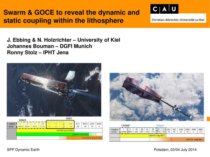
Swarm & GOCE to reveal the dynamic and static coupling within the lithosphere. J. Ebbing & N. Holzrichter – University of Kiel Johannes Bouman – DGFI Munich Ronny Stolz – IPHT Jena. SPP Dynamic Earth Potsdam, 03/04 July 2014. Modelling Concept. Crust. Moho.

E N D
Swarm & GOCE to reveal the dynamic and static coupling within the lithosphere J. Ebbing & N. Holzrichter – University of Kiel Johannes Bouman – DGFI Munich Ronny Stolz – IPHT Jena SPP Dynamic Earth Potsdam, 03/04 July 2014
ModellingConcept Crust Moho Lithospheric mantle 1315°C LAB 1315°C Asthenospheric mantle
SWARM Curie temperature isotherm 580°C Crust Moho 580°C Lithospheric mantle 1315°C LAB 1315°C Asthenospheric mantle
SWARM Gravity gradients (GOCE) Curie temperature isotherm Crust 580°C Moho 580°C Δρ Lithospheric mantle 1315°C LAB 1315°C Asthenospheric mantle
SWARM Gravity gradients (GOCE) (GOCE,GRACE) Curie temperature isotherm Crust 580°C Moho 580°C Δρ GOCE gradients ρ(T,C) Lithospheric mantle Δρ 1315°C LAB 1315°C Gravity, Geoid ρ(T,C) Asthenospheric mantle
GOCE data @ satellite altitude / Earth’s surface • Signal @ satellite altitude is smooth • Downward continuation enhances signal power & details
GOCE data @ satellite altitude / Earth’s surface • Downward continuation also amplifies noise • Effective resolution of data does not change • Omission error becomes much larger (mainly high frequency topography) VZZ degree RMS h = 0 & 260 km GOCO03S VZZ signal & error, L = 225 For model inversion it is probablybest to use data close to theiroriginal point of acquisition.
Moho depth by gravityinversion Inversion: Gz >90 km Z0=30 km Dr= 350 kg/m3
Moho depth by gravityinversion • - satelliteresiduals - Inversion: Gz >90 km Z0=30 km Dr= 350 kg/m3
Moho depth by satellitegravity gradient inversion Inversion Gzz=Full Z0=30 km Dr= 350 kg/m3
Sensitivityofsatellite gradients Sensitivitykernels for sphericalgravity gradients Z. Martinec 2013
... with present satellitesØrsted and CHAMP ...N = 60, resolution: 670 km ... and with SwarmN = 133, resolution: 300 km Improvement of Lithospheric Field Model Before Ørsted ...N = 30, resolution: 1330 km Magnetic field of Earth’s crustradial component at 10 km altitude
Sphericalmodellingtools The formula to calculate gravity gradient tensor of a spherical prism (Asgharzadeh et al., 2007), along with adaptive integration method (Li et al., 2011) was used in software package called tesseroids-1.1 (Uiedaet al., 2011; Uieda, 2013). By Poisson’s relation (Blakely, 1995) the magnetic field is mathematically equivalent to the gradient of a gravity field. Therefore, tesseroidswas modified to calculate a magnetic field. To this end the Earth crust is modelled by spherical prisms with prescribed magnetic susceptibility and remanent magnetization. Induced magnetizations are then derived from product of the chosen main field model (such as International Geomagnetic Reference Field) and the corresponding tesseroid susceptibilities. Remanent magnetization vectors are directly set. = + Poisson’s relation Magnetization of a tesseroid.
Numericalmethods in comparison (Baykiev 2014) • TesseroidsSphericalcaps • Input: Crust1.0 • Susceptibility of the whole crust – 0.04 SI • Ambient field – IGRF11 • Grid resolution – 2x2 deg • Grid altitude – 400 km (also in Purucker et al. 2002)
A study area • Why Greenland? • Little geophysical data available • Mass estimates of changing ice sheets necessary for climate models • Coupling with physical state of lithosphere essential to estimate dynamic behaviour • Role of Iceland hotspot track?
Summary • Analysis of satellite gravity data: • lithospheric structure • Ice thickness vs. crustal thickness • dynamic vs. static components • Analysis of satellite magnetic data: • Characterization of magnetic crustal thickness • Normalized source strength for describing tectonic domains • Interpretation with DTU & GEUS • Implications for rheology • Technical challenges: • Magnetic gradients along the track (with DTU) • Tesseroids for complete magnetic tensor modelling (with NGU) • Implementation of invariant analysis in inverse and forward modelling