The Control Chart for Attributes

1. The Control Chart for Attributes Topic • The Control charts for attributes • The p and np charts • Variable sample size • Sensitivity of the p chart

2. Types of Data • Variable data • Product characteristic that can be measured • Length, size, weight, height, time, velocity • Attribute data • Product characteristic evaluated with a discrete choice • Good/bad, yes/no

3. The Control Chart for Attributes • In a control chart for variables, quality characteristic is expressed in numbers. Many quality characteristics (e.g., clarity of glass) can be observed only as attributes, i.e., by classifying into defectives and non-defectives. • If many quality characteristics are measured, a separate control chart for variable will be needed for each quality characteristic. A control chart for attribute is a cheaper alternative. It records an item defective if any specification is not met and non-defective if all the specifications are met.

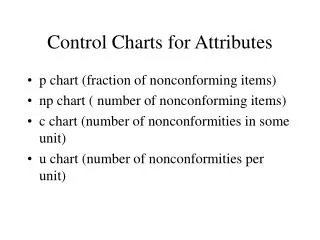
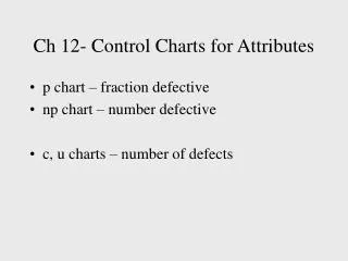
4. The Control Chart for Attributes • The cost of collecting data for attributes is less than that for the variables • There are various types of control charts for attributes: • Thep chart for the fraction rejected • The np chart for the total number rejected • The c chart for the number of defects • The u chart for the number of defects per unit

5. The Control Chart for Attributes • Poisson Approximation: • Occurrence of defectives may be approximated by Poisson distribution • Let n = number of items and p = proportion of defectives. Then, the expected number of defectives, • Once the expected number of defectives is known, the probability of c defectives as well as the probability of c or fewer defectives can be obtained from Appendix 4

6. The Control Chart for Fraction Rejected The p Chart: Constant Sample Size Steps 1. Gather data 2. Calculate p, the proportion of defectives 3. Plot the proportion of defectives on the control chart 4. Calculate the centerline and the control limits (trial) 5. Draw the centerline and control limits on the chart 6. Interpret the chart 7. Revise the chart

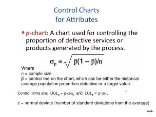
7. The Control Chart for Fraction Rejected The p Chart: Constant Sample Size • Step 4: Calculating trial centerline and control limits for the p chart

8. The Control Chart for Fraction Rejected The p Chart: Constant Sample Size • Step 6: Interpretation of the p chart • The interpretation is similar to that of a variable control chart. there should be no patterns in the data such as trends, runs, cycles, or sudden shifts in level. All of the points should fall between the upper and lower control limits. • One difference is that for the p chart it is desirable that the points lie near the lower control limit • The process capability is the centerline of the p chart

9. The Control Chart for Fraction Rejected The p Chart: Constant Sample Size • Step 7: Revised centerline and control limits for the p chart

10. The Control Chart for Fraction Rejected The np Chart • The np chart construction steps are similar to those of the p chart. The trial centerline and control limits are as follows:

11. Variable Sample SizeChoice Between the p and np Charts • If the sample size varies, p chart is more appropriate • If the sample size is constant, np chart may be used

12. Sensitivity of the p Chart • Smaller samples are • less sensitive to the changes in the quality levels and • less satisfactory as an indicator of the assignable causes of variation • Smaller samples may not be useful at all e.g., if only 0.1% of the product is rejected • If a control chart is required for a single measurable characteristic, chart will give useful results with a much smaller sample.

13. Example 1: A manufacturer purchases small bolts in cartons that usually contain several thousand bolts. Each shipment consists of a number of cartons. As part of the acceptance procedure for these bolts, 400 bolts are selected at random from each carton and are subjected to visual inspection for certain non-conformities. In a shipment of 10 cartons, the respective percentages of rejected bolts in the samples from each carton are 0, 0, 0.5, 0.75, 0,2.0, 0.25, 0, 0.25, and 1.25. Does this shipment of bolts appear to exhibit statistical control with respect to the quality characteristics examined in this inspection?

14. Example 2: An item is made in lots of 200 each. The lots are given 100% inspection. The record sheet for the first 25 lots inspected showed that a total of 75 items did not conform to specifications. a. Determine the trial limits for an np chart. b. Assume that all points fall within the control limits. What is your estimate of the process average fraction nonconforming ? c. If this remains unchanged, what is the probability that the 26th lot will contain exactly 7 nonconforming units? That it will contain 7 or more nonconforming units? (Hint: use Poisson approximation and Appendix 4)

15. Example 3: A manufacturer wishes to maintain a process average of 0.5% nonconforming product or less. 1,500 units are produced per day, and 2 days’ runs are combined to form a shipping lot. It is decided to sample 250 units each day and use an np chart to control production. (a) Find the 3-sigma control limits for this process. (b) Assume that the process shifts from 0.5 to 4% nonconforming product. Appendix 4 to find the probability that the shift will be detected as the result of the first day’s sampling after the shift occurs. (c) What is the probability that the shift described in (b) will be caught within the first 3 days after it occurs?

16. The Control Chart for Attributes Topic • The p chart for the variable sample size • Calculating p chart limits using nave • Percent nonconforming chart • The c chart • The u chart with constant sample size • The u chart with variable sample size

17. The Control Chart for Fraction Rejected The p Chart: Variable Sample Size • When the number of items sampled varies, the p chart can be easily adapted to varying sample sizes • If the sample size varies • the control limits must be calculated for each different sample size, changing the n in the control-limit formulas each time a different sample size is taken. • calculating the centerline and interpreting the chart will be the same

18. The Control Chart for Fraction Rejected The p Chart: Variable Sample Size Steps 1. Gather data 2. Calculate p, the proportion of defectives 3. Plot the proportion of defectives on the control chart 4. Calculate the centerline. For each sample calculate a separate pair of control limits. 5. Draw the centerline and control limits on the chart 6. Interpret the chart

19. The Control Chart for Fraction Rejected The p Chart: Variable Sample Size • Step 4: Calculate the centerline. For each sample calculate a separate pair of control limits. Let m = number of samples.

20. The Control Chart for Fraction Rejected The p Chart: Variable Sample Size • Step 6: Interpretation of the p chart • The interpretation is similar to that of a variable control chart. there should be no patterns in the data such as trends, runs, cycles, or sudden shifts in level. All of the points should fall between the upper and lower control limits. • One difference is that for the p chart it is desirable that the points lie near the lower control limit • The process capability is the centerline of the p chart

21. The Control Chart for Fraction Rejected The p Chart: Variable Sample Size Calculation of Control Limits Using nave • The calculation of control limits for the p chart with variable sample size can be simplified with the use of nave • The value nave can be found by summing up the individual sample sizes and dividing by the total number of times samples were taken:

22. The Control Chart for Fraction Rejected The p Chart: Variable Sample Size Calculation of Control Limits Using nave • The value nave can be used whenever the individual sample sizes vary no more than 25% from the calculated nave • The advantage of using is that there will be a single pair of upper and lower control limits

23. The Control Chart for Fraction Rejected The p Chart: Variable Sample Size Calculation of Control Limits Using nave • However, if the control limits are computed using the nave the points inside and outside the control limits must be interpreted with caution: • See the control limit formula - for a larger sample, the control limits are narrower and for a smaller sample, the control limits are wider • So, if a larger sample produces a point inside the upper control limit computed using nave, the point may actually be outside the upper control limit when the upper control limit is computed using the individual sample size

24. The Control Chart for Fraction Rejected The p Chart: Variable Sample Size Calculation of Control Limits Using nave • Similarly, if a smaller sample produces a point outside the upper control limit computed using nave, the point may actually be inside the upper control limit when the upper control limit is computed using the individual sample size • If a larger sample produces a point inside the upper control limit, the individual control limit should be calculated to see if the process is out-of-control • If a smaller sample produces a point outside the upper control limit, the individual control limit should be calculated to see if the process is in control

25. The Control Chart for Fraction Rejected The p Chart: Variable Sample Size Calculation of Control Limits Using nave • The previous discussion leads to the following four cases: • Case I: The point falls inside the UCLp and nind < nave • No need to check the individual limit • Case II: The point falls inside the UCLp and nind > nave • The individual limits should be calculated • Case III: The point falls outside the UCLp and nind > nave • No need to check the individual limit • Case IV: The point falls outside the UCLp and nind < nave • The individual limits should be calculated • Check points: All the points near UCL. Check only the points which are near UCL.

26. The Control Chart for Fraction Rejected The Percent Nonconforming ChartConstant Sample Size • The centerline and control limits for the percent nonconforming chart

27. The Control Chart for NonconformitiesThe c and u charts • Defective and defect • A defective article is the one that fails to conform to some specification. • Each instance of the article’s lack of conformity to specifications is a defect • A defective article may have one or more defects

28. The Control Chart for NonconformitiesThe c and u charts • The np and c charts • Both the charts apply to total counts • The np chart applies to the total number of defectivesin samples of constant size • The c chart applies to the total number of defects in samples of constant size • The p and u charts • The p chart applies to the proportion of defectives • The u chart applies to the number of defects per unit • If the sample size varies, the p and u charts may be used

29. The Control Chart for Counts of Nonconformities The c Chart: Constant Sample Size • The number of nonconformities, or c, chart is used to track the count of nonconformities observed in a single unit of product of constant size. • Steps 1. Gather the data 2. Count and plot c, the count of nonconformities, on the control chart. 3. Calculate the centerline and the control limits (trial) 4. Draw the centerline and control limits on the chart 5. Interpret the chart 6. Revise the chart

30. The Control Chart for Counts of Nonconformities The c Chart: Constant Sample Size • Step 3: Calculate the centerline and the control limits (trial)

31. The Control Chart for Counts of Nonconformities The c Chart: Constant Sample Size • Step 5: Interpretation of the c chart • The interpretation is similar to that of a variable control chart. there should be no patterns in the data such as trends, runs, cycles, or sudden shifts in level. All of the points should fall between the upper and lower control limits. • One difference is that for the c chart it is desirable that the points lie near the lower control limit • The process capability is the centerline of the c chart

32. The Control Chart for Counts of Nonconformities The c Chart: Constant Sample Size • Step 6: Revised centerline and control limits for the c chart

33. Number of Nonconformities Per Unit The u Chart: Constant Sample Size • The number of nonconformities per unit, or u chart is used to track the number of nonconformities in a unit. • Steps 1. Gather the data 2. Count and plot u, the number of nonconformities per unit, on the control chart. 3. Calculate the centerline and the control limits (trial) 4. Draw the centerline and control limits on the chart 5. Interpret the chart 6. Revise the chart

34. Number of Nonconformities Per Unit The u Chart: Constant Sample Size • Step 2: Count and plot u, the number of nonconformities per unit, on the control chart.

35. Number of Nonconformities Per Unit The u Chart: Constant Sample Size • Step 3: Calculate the centerline and the control limits (trial)

36. Number of Nonconformities Per Unit The u Chart: Constant Sample Size • Step 6: Revise the chart

37. Number of Nonconformities Per Unit The u Chart: Variable Sample Size • When the sample size varies, compute • either the individual control limits • or a control limit using nave • When using nave no individual sample size may vary more than 25% from nave

38. The Control Chart for NonconformitiesThe c and u charts • As the Poisson distribution is not symmetrical, the upper and lower 3-sigma limits do not correspond to equal probabilities of a point on the control chart falling outside limits. To avoid the problem with asymmetry, the use of 0.995 and 0.005 limits has been favored • If the distribution does not follow Poisson law, actual standard deviation may be greater than and, therefore, 3-sigma limit may actually be greater than limit obtained from the formula

39. Example 4: The following are data on 5-gal containers of paint. If the color mixture of the paint does not match the control color, then the entire container is considered nonconforming and is disposed of. Since the amount produced during each production run varies, use nave to calculate the centerline and control limits for this set of data. Carry calculations to four decimal places. Remember to Round nave to a whole number; you can’t sample part of a 5-gal pail. Production run 1 2 3 4 5 6 Number inspected 2,524 2,056 2,750 3,069 3,365 3,763 Number defective 30 84 76 108 54 29 Production run 7 8 9 10 11 12 Number inspected 2,675 2,255 2,060 2,835 2,620 2,250 Nunmber defective 20 25 48 10 86 25

41. Example 5: A c chart is used to monitor the number of surface imperfections on sheets of photographic film. The chart presently is set up based on of 2.6. (a) Find the 3-sigma control limits for this process. (b) Use Appendix 4 to determine the probability that a point will fall outside these control limits while the process is actually operating at a c of 2.6. (c) If the process average shifts to 4.8, what is the probability of not detecting the shift on the first sample taken after the shift occurs?

42. Example 6: A shop uses a control chart on maintenance workers based on maintenance errors per standard worker-hour. For each worker, a random sample of 5 items is taken daily and the statistic c/nis plotted on the worker’s control chart where c is the count of errors found in 5 assemblies and n is the total worker-hours required for the 5 assemblies. (a) After the first 4 weeks, the record for one worker is c=22 and n=54. Determine the central line and the 3-sigma control limits. (b) On a certain day during the 4-week period, the worker makes 2 errors in 4,3 standard worker-hour. Determine if the point for this day falls within control limits.

43. Reading and Exercises • Chapter 9: • Reading pp. 404-447 (2nd ed.) • Problems 5, 10 (solve with and without nave), 11, 13, 14, 19, 20, 23, 25 (2nd ed.) • Reading pp. 414-453 (3rd ed.) • Problems 5, 10 (solve with and without nave), 11, 13, 14, 19, 20, 23, 25 (2nd ed.)

44. Acceptance Sampling Outline • Sampling • Some sampling plans • A single sampling plan • Some definitions • Operating characteristic curve

45. Necessity of Sampling • In most cases 100% inspection is too costly. • In some cases 100% inspection may be impossible. • If only the defective items are returned, repair or replacement may be cheaper than improving quality. But, if the entire lot is returned on the basis of sample quality, then the producer has a much greater motivation to improve quality.

46. Some Sampling Plans • Single sampling plans: • Most popular and easiest to use • Two numbers n and c • If there are more than c defectives in a sample of size n the lot is rejected; otherwise it is accepted • Double sampling plans: • A sample of size n1 is selected. • If the number of defectives is less than or equal to c1 than the lot is accepted. • Else, another sample of size n2 is drawn. • If the cumulative number of defectives in both samples is more than c2 the lot is rejected; otherwise it is accepted.

47. Some Sampling Plans • A double sampling plan is associated with four numbers: • The interpretation of the numbers is shown by an example: 1. Inspect a sample of size 20 2. If the sample contains 3 or less defectives, accept the lot 3. If the sample contains more than 5 defectives, reject the lot.

48. Some Sampling Plans 4. If the sample contains more than 3 and less than or equal to 5 defectives (i.e., 4 or 5 defectives), then inspect a second sample of size 10 5. If the cumulative number of defectives in the combined sample of 30 is not more than 5, then accept the lot. 6. Reject the lot if there are more than 5 defectives in the combined lot of 30 • Double sampling plans may be extended to triple sampling plans, which may also be extended to higher order plans. The logical conclusion of this process is the multiple or sequential sampling plan.

49. Some Sampling Plans • Multiple sampling plans • The decisions (regarding accept/reject/continue) are made after each lot is sampled. • A finite number of samples (at least 3) are taken • Sequential sampling plans • Items are sampled one at a time and the cumulative number of defectives is recorded at each stage of the process. • Based on the value of the cumulative number of defectives there are three possible decisions at each stage: • Reject the lot • Accept the lot • Continue sampling

50. Some Sampling Plans • Multiple sampling and sequential sampling are very similar. Usually, in a multiple sampling plan the decisions (regarding accept/reject/continue) are made after each lot is sampled. On the other hand, in a sequential sampling plan, the decisions are made after each item is sampled. In a multiple sampling, a finite number of samples (at least 3) are taken. A sequential sampling may not have any limit on the number of items inspected.