Exponential Functions as Mathematical Models

1. Exponential Functions as Mathematical Models By Dr. Julia Arnold and Ms. Karen Overman using Tan’s 5th edition Applied Calculus for the managerial , life, and social sciences text

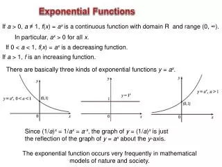
2. Exponential Growth There are some real life situations that can be modeled by the exponential functions previously studied. Recall in Section 5.3 on compound interest we looked at the formula for interest compounded continuously, . This model is an example of exponential growth. The general equation for exponential growth is , where Q(t) is the amount present at any time t, is the initial amount (or P, the amount invested in the interest example) and k is a positive constant,called the growth constant (or r, the interest rate in the interest example).

3. Exponential Growth Model Q(t) = the amount at any time, t = the initial amount k = the growth constant t = the time You should note that at time t = 0, Q(0) = , which is the initial amount and as t increases without bound, Q(t) also increases without bound.

4. Now let’s consider the rate of change of Q(t) otherwise known as the derivative of Q(t). Since, The derivative will be: If , this says that the rate of growth at any time, t is directly proportional to the amount, Q(t). Thus when a function has this quality, that the rate of growth is directly proportional to the amount, it is said to exhibit exponential growth.

5. It’s amazing how mathematics can attach formulas to real life examples. Example 1: Exponential Growth The growth rate of the bacterium E-Coli, is proportional to its size. Under ideal laboratory conditions, when this bacterium is grown in a nutrient broth medium, the number of cells in a culture doubles approximately every 20 min. If the initial cell population is 100, determine the function Q(t) that expresses the exponential growth of the number of cells of this bacterium as a function of time t in minutes.

6. Example 1: Exponential Growth The growth rate of the bacterium E-Coli, is proportional to its size. Under ideal laboratory conditions, when this bacterium is grown in a nutrient broth medium, the number of cells in a culture doubles approximately every 20 min. If the initial cell population is 100, determine the function Q(t) that expresses the exponential growth of the number of cells of this bacterium as a function of time t in minutes. Key words: growth ratewould refer to the derivative of Q or Q’.

7. Example 1: Exponential Growth The growth rate of the bacterium E-Coli, is proportional to its size. Under ideal laboratory conditions, when this bacterium is grown in a nutrient broth medium, the number of cells in a culture doubles approximately every 20 min. If the initial cell population is 100, determine the function Q(t) that expresses the exponential growth of the number of cells of this bacterium as a function of time t in minutes. Key words: growth ratewould refer to the derivative of Q or Q’. The growth rate of the bacterium E-Coli, is proportional to its sizeimplies the equation: Q ‘(t) = k Q(t) which in turn implies the exponential growth equation: Q(t) = Q0ekt

8. Example 1: Exponential Growth The growth rate of the bacterium E-Coli, is proportional to its size. Under ideal laboratory conditions, when this bacterium is grown in a nutrient broth medium, the number of cells in a culture doubles approximately every 20 min. If the initial cell population is 100, determine the function Q(t) that expresses the exponential growth of the number of cells of this bacterium as a function of time t in minutes. Q(t) = Q0ekt is our equation where Q0 represents the amount present at time t = 0, also known as the initial amount. Q(t) = 100ekt

9. Example 1: Exponential Growth The growth rate of the bacterium E-Coli, is proportional to its size. Under ideal laboratory conditions, when this bacterium is grown in a nutrient broth medium, the number of cells in a culture doubles approximately every 20 min. If the initial cell population is 100, determine the function Q(t) that expresses the exponential growth of the number of cells of this bacterium as a function of time t in minutes. Since the number of cells doubles every 20 min, this means Q(t)= 200 when t = 20. 200 = 100ek20 Now we can solve for k.

10. For Example 1, we are trying to determine the function Q(t) that expresses the exponential growth of the number of cells of this bacterium as a function of time t in minutes. 200 = 100ek20 2 = e20k ln2 = lne20k ln2 = 20k Now that we know k, we have an equation that describes the growth of the bacteria for this problem. Q(t)= 100 e.035t Part B: How long will it take for a colony of 100 cells to increase to a population of 1 million? 1,000,000= 100 e.035t and we want to find the time t. This is another exponential equation which requires logs to solve.

11. 1,000,000= 100 e.035t10000 = e.035tln(10000) = ln (e.035t)ln(10000) = .035t 263.15 min is 4.38 hours Part C: If the initial cell population were 1000, how would this alter our model? This equation, 200 = 100ek20, would become 2000=1000e20k, which would still yield 2=e20k, so k would remain the same value. Part B would change to 1,000,000 = 1000e.035t which would become ln1000/.035 ~ 197.36~3.28 hours

12. Exponential Decay Radioactive substances decay exponentially. These substances obey the rule: Q(t)= Q0e-kt where Q0 is the initial amount present and k is a suitable positive constant. With the exponential decay model, when t = 0, Q(t) = Q0 just like the previous model, but as t increases without bound Q(t) approaches 0. This is a decreasing function since the exponent on e is negative. The half-life of a radioactive substance is the time required for a given amount to be reduced by ½.

13. Example 2: Fossils discovered in South America contain 5% of the Carbon 14 they originally contained. If you know that the half-life of Carbon 14 is 5770 years, calculate the age of the fossils. Solution: If you know the half-life of Carbon 14 is 5770 years, then when t = 5770 years the amount of Carbon 14 is ½ the original amount. Say the original amount is Q0 Then ½ the original amount is ½ Q0

14. Example 2: Fossils discovered in South America contain 5% of the Carbon 14 they original contained. If you know that the half-life of Carbon 14 is 5770 years, calculate the age of the fossils. Solution: If you know the half-life of Carbon 14 is 5770 years, then when t = 5770 years the amount of Carbon 14 is ½ the original amount. Say the original amount is Q0 Then ½ the original amount is ½ Q0 Now solve for k. Thus, ½ Q0 = Q0e-k5770 ½ = e-k5770 ln (½) = ln(e-k5770 ) Or k = ln (½)/-5770=0.00012 ln (½) = -5770k

15. Example 2 continued. Now that we know k=0.00012, we can substitute it back into the exponential decay model and use that model to answer the question. Q(t)= Q0e-0.00012t The question was how old are the fossils if they contain 5% of the original amount of Carbon 14. Here we know the amount is 5% of the original amount or 0.05Q0 . Substitute this in for Q(t) and solve for t. 0.05 Q0=Q0e-0.00012t Or t = ln0.05/-0.00012 t = 24,964 years 0.05 =e-0.00012t ln0.05 =lne-0.00012t ln 0.05 = -0.00012t

16. Example 3: Atmospheric Pressure If the temperature is constant, then the atmospheric pressure P ( in pounds per square inch) varies with the altitude above sea level h in accordance with the law, P = p0e-kh where p0 is the atmospheric pressure at sea level and k is a constant. If the atmospheric pressure is 15 lb/in2 at sea level and 12.5 lb/in2 at 4000 ft, find the atmospheric pressure at an altitude of 12,000 ft. How fast is the atmospheric pressure changing with respect to altitude at an altitude of 12,000 ft? Solution: Begin with the generic equation and substitute what we know.

17. Example 3: Atmospheric Pressure If the temperature is constant, then the atmospheric pressure P ( in pounds per square inch) varies with the altitude above sea level h in accordance with the law, P = p0e-kh where p0 is the atmospheric pressure at sea level and k is a constant. If the atmospheric pressure is 15 lb/in2 at sea level and 12.5 lb/in2 at 4000 ft, find the atmospheric pressure at an altitude of 12,000 ft. How fast is the atmospheric pressure changing with respect to altitude at an altitude of 12,000 ft? Solution: Begin with the generic equation and substitute what we know. This tells us p0 = 15 lb/in2 P = 15e-kh

18. Example 3: Atmospheric Pressure If the temperature is constant, then the atmospheric pressure P ( in pounds per square inch) varies with the altitude above sea level h in accordance with the law, P = p0e-kh where p0 is the atmospheric pressure at sea level and k is a constant. If the atmospheric pressure is 15 lb/in2 at sea level and 12.5 lb/in2 at 4000 ft, find the atmospheric pressure at an altitude of 12,000 ft. How fast is the atmospheric pressure changing with respect to altitude at an altitude of 12,000 ft? Solution: P = 15e-kh Now we substitute 12.5 for P and 4000 for h. 12.5 = 15e-k4000

19. 12.5 = 15e-k4000 Now the equation is P = 15 e-.000045h Find the atmospheric pressure at an altitude of 12,000 ft P = 15 e-.000045(12000)~8.7 lb/in2

20. The second part of the question asks: How fast is the atmospheric pressure changing with respect to altitude at an altitude of 12,000 ft? This is asking for the rate of change, P’ at h = 12,000 The minus tells us the pressure is dropping.

21. You should use these examples as a guide when working the practice problems. Below is some additional information you may need for the practice exercises. Use this information as appropriate. The half-life of radium is know to be approximately 1600 years. Carbon 14 has a half-life of 5770 years.