Download
1 / 22
220 likes | 446 Views
Extraction of Salient Contours in Color Images. Vonikakis Vasilios, Ioannis Andreadis and Antonios Gasteratos . Democritus University of Thrace 2006 . Presentation Overview. Problem definition Biological background Description of the model Results Conclusions.

E N D
Extraction of Salient Contours in Color Images Vonikakis Vasilios, Ioannis Andreadis and Antonios Gasteratos Democritus University of Thrace 2006
Presentation Overview • Problem definition • Biological background • Description of the model • Results • Conclusions
Definitions: Salient Contours Salient contours: The most evident contours that draw the attention of an observer Problem definition
Applications of salient contours • Create the ‘primal sketch’ of the image • Filter the optical data and keep only the significant information • Reduce the amount of visual information that a visual system processes Problem definition
The Human Visual System Optic nerve Visual Cortex V1, V2… Retina (ganglion cells) light Biological background
R+G-B G-R -R-G-B B-R-G R-G R+G+B Black-White Blue-Yellow Red-Green Double opponent cells • They are located in area V1 • Two chromatic and one achromatic • They have a center-surround receptive field • They receive opposite signal to center and surround • They respond only to changes between center and surround – edges detectors Biological background
The primary visual cortex V1 • The visual cortex analyses the retinal output in 3 different maps: • Color (double-opponent cells) • motion-depth • orientation of edges • At every position of the visual field, the V1 has cells (orientation filters) of all possible orientations Biological background
Favorite connections of a horizontal orientation cell Connection of orientation cells • Orientation cells prefer to be connected with others that create co-circular paths • This favors the smooth continuity of contours Biological background
Block diagram of the model Extraction of color edges Salient Contours network Input Image Description of the model
9x9 mask Center Surround Extracting color edges • Similar to the double-opponent cells of V1 Description of the model
max { RG, BY, BW } Extracting color edges BY RG BW Description of the model
60 kernels • 10×10 pixel size • 12 orientations • all possible positions within every orientation Orientation filters Objective: to encode the orientation of the edges • The image is divided to 10×10 non-overlapping regions • For every region all 60 kernels are convolved • The higher response defines the kernel that best describes the orientation of the region Description of the model
Kernel 24:75° Kernel 19:135° Encoded edges Color edge image Image with oriented filters Description of the model
Kernel 6 Kernel 54 Kernel 17 j n n n n n i m n n n n n n Computing the connection matrix • We have calculated the connection matrix of all the 60 kernels, in a 5×5 kernel neighborhood Connection matrix: weight [60] [5] [5] [60] weight [m] [ i ] [ j ] [n] : connection from kernel ‘m’ in the center of the 5×5 region, to kernel ‘n’ in the (i,j) position Description of the model
Basic influence equation of kernel m (i,j) to kernel n outn(t) = outn(t-1) + weightm(i,j)→n× outm(t) Influence between kernels • If weightm(i,j)→n>0 (kernel m is in the favorite curves of n) the influence is excitatory (outn(t)>outn(t-1)) • If weightm(i,j)→n<0 (kernel m is not in the favorite curves of n) the influence is inhibitory (outn(t)<outn(t-1)) Description of the model
Lobe 2 Lobe 1 F • L1: total excitatory influence to Lobe 1 • L2: total excitatory influence to Lobe 2 • inh: total inhibitory influence k Activation function of kernel k • Only the kernels with equal excitation in both lobes achieve high output • This favors the good continuation of salient contours Description of the model
Oriented filters t=0 t=19 t=9 t=1 Iterations • Salient contour kernels gradually increase their values • Kernels of non-salient contours gradually decrease their values • Usually 10 iterations are necessary Description of the model
Results Original image Color edges Salient contours 700×700: 2.7 sec Results 700×576: 2.3 sec
More results Original image Color edges Salient contours 1000×768: 4.8 sec 1000×768: 4.8 sec Results
More results Original image Color edges Salient contours 500×750: 2.1 sec Results 672×496: 1.8 sec
Conclusions • The proposed extraction of edges exhibits better results, especially for isoluminant areas, than the gradient of R,G and B • The proposed kernel set is an adequate way of coding the orientation of edges • The proposed method successfully extracts some of the most salient contours of the image • The execution time of the method when executed by a conventional PC is small compared to other saliency algorithms in the field