Download
1 / 29
310 likes | 474 Views
Spatial analysis of geochemical data. Shawn Laffan. Hotspot identification. Where are the regions of excess element abundance? Greater than expected Anomalously high Where are the regions of less than expected abundance?. Hotspot identification.

E N D
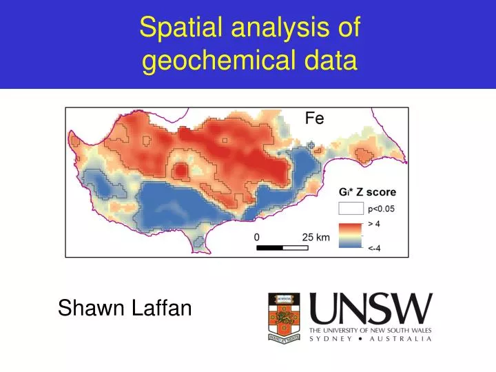
Spatial analysis of geochemical data Shawn Laffan
Hotspot identification • Where are the regions of excess element abundance? • Greater than expected • Anomalously high • Where are the regions of less than expected abundance?
Hotspot identification • Need quantitative comparison within and between data sets • Looking for clusters • Moving window analyses • Geographically local
Tobler’s First Law • That everything is related to everything else, but that near things are more related than those far apart
Hotspot identification • Spatial scale • Spatial extent • Spatial non-stationarity • Significance
Getis-Ord hotspot statistic Sum weighted valuesin window Subtract sum of weights * mean (expected value) Divide by standard deviation andcorrect for weights used in window
Getis-Ord hotspot statistic • Positive for samples that are, on average, above the mean • Negative if below the mean • Z-score • >+1.96 significant hotspot • <-1.96 significant coldspot
Choice of weights (sample window) • Binary • Resultant surfaces can have abrupt changes • Continuous • Smoother surfaces • Gaussian – asymptotes to zero • IDW - asymptotes to zero • Bisquare – decays to zero
Gi* analyses • Fe, Ni, Pb, Cu, Li, Cr, Ce/Li, Cr/Fe • log10 scaled • 1 km resolution rasters • Maximum value if >1 point in a cell
Gi* analyses • Bisquare weights with 4 bandwidths • 2, 3, 4 & 5 km • Identified “optimal” scale at each location • Bandwidth with most extreme Gi* score
Visual comparison with lithology and landform • Landform (terrain): • Slope gradient • Longitudinal curvature • Rate of change of slope gradient • +ve = Convex up = spur line • -ve = Concave up = break of slope • 0 = Planar • Circular analysis windows • Radii: 1 & 5 km (local & regional) • SRTM 3 arc second DEM
Conclusions • Hotspots broadly consistent with lithology • Weak association with landform • and terrain is controlled by lithology... • Finer detail possibly due to other causes • e.g. Pb & anthropogenic activities
Jenny’s CLORPT model • Soil = f (Climate, Organic, Relief, Parent material, Time)
Future • Use alternate expected values • Environmental guidelines • Economic grade • Analyse as indicators • Binary above/below threshold