Download
1 / 35
350 likes | 444 Views
Practicalities of Digital Control. A Survey. The Overall System. The individual controllers The interconnection The central computer or computers The transducers and actuators. The individual controllers. P L C General-purpose controllers Purpose-built. More on the P L C.

E N D
Practicalities of Digital Control A Survey
The Overall System • The individual controllers • The interconnection • The central computer or computers • The transducers and actuators
The individual controllers • P L C • General-purpose controllers • Purpose-built
More on the P L C • Probably still ‘ladder logic’ -- good for on-off control but cumbersome for analogue --but ... • Can incorporate analogue I/O • Can often include p.i.d. controller blocks and routines in high-level languages • Most modern PLC types can be interfaced to a SCADA system
Traditional example -- Mitsubishi F1/F2 • Basically ladder logic • Can do analogue quantities, but awkward • Good at on -- off control • An analogue ladder example follows • More modern networkable PLCs will be described in a later lecture
General-purpose Controllers • Most common type is PID but other strategies possible • Parameters can be changed/downloaded by/from SCADA system • Self-tuning types becoming more popular but care is still needed in their use • Less good at on-off than the PLC • Better at ‘analogue’ control
DSP Possibility • Can be based on DSP Chips • Very fast micros optimised for multiply-and-add ... the sums of digital control • Some can operate in floating-point • Serial interface to I/O
How fast shall we sample ? • Shannon/Nyquist Theorem -- we must sample at least twice the highest frequency present if we are not to lose information • Actually we need to sample faster than this to avoid aliasing and because of noise • 10 - 20 x highest frequency of interest is usual
Why ? • Less than 10 x means it is difficult to produce an effective anti-aliasing filter • More than 20 x leads to a double penalty ... • We have to do the sums faster ... • ... and more accurately if they are to work ! • But what is this aliasing thing ?
Suppose we sample this signal every 14 s x 10 x x 5 0 x x -5 x x -10 0 20 40 60 80 100
“I’ve got aliasing, doctor.” • We have ‘found’ a sine wave of much lower frequency than the actual one. • The system may be able to respond to the lower frequency one ... • ... even if the original was too fast for it to respond to.
“I’ll give you a prescription for ...” • Some effective screening (the high-frequency signal is likely to be the mains or Radio 1/2/3/4/5/etc) • An analogue low-pass filter on the inputs
The anti-aliasing filter • Has to be analogue (it would itself be at the risk of aliasing if it were digital !) • It must not appreciably affect signals within the normal frequency range of the controller but it must effectively remove everything above half the sampling frequency. • The faster we sample, the easier it is to remove the aliasing signals.
A Sampling-rate Example • Controller 0.1s + 1 +2/s • We have already digitised with a sampling interval of 0.05 s • We will see what happens with 0.25 s ... • ... and 0.01 s. • Using the simple substitution.
We obtain with Ts = 0.25 s ... • 1.9 - 1.8z-1 + 0.4z-2 • ----------------------- • 1 - z-1 • This one causes very serious degradation of performance -- if not actual instability
What is happening ? • The problem is that by sampling we are producing a Transport lag • We remember from Analogue Control that a Transport Lag is a pure time delay .. • ... and that it reduces system stability by increasing the phase lag in the loop. • We introduce one by sampling ...
What is happening -- Continued • ... because an event happening during a sampling interval is only detected at the next sampling instant. • So the delay in detecting it can be anything between zero and a full sampling interval .. • .. so it is Ts/2 on average. • This is the effective extra transport lag introduced by sampling.
...So let us use Ts = 0.02 s ... • 11.02 - 21z-1 + 10z-2 • --------------------------- • 1 - z-1 • If we do not do the sums very accurately, we entirely lose the integral term !
Ts = 0.02 s .. A Consequence • We will lose the integral term entirely if we use 8-bit arithmetic. • I will do the sum ... • ... in which we are only allowed integer numbers between 0 and 255 (or probably between -128 and +127 in practice)
Interconnection • Multi-line bus (VME etc) • Parallel or serial • Two-wire (FIELDBUS etc) • Systems often combine hardware and software
Analogue Interfaces • Voltage ranges (often 0 -> 10 V or -10 -> 10 V) • Current loop (usually 4-20 mA) • So e.g. for 8-bit, 4 mA converts to 0 and 20 mA converts to 25510 • What would the values be for 12 and 16 bits ?
Arithmetic • Now normally floating-point within the controller • Fixed-point arithmetic is still used in some low-cost (often mass-produced) equipment • It saves hardware cost but incurs extra development time • Input and output are still fixed-point
Precision • 8-bit I/O restricts us to 0-255 decimal • 12-bit often used in ‘good’ systems
Supervisory Control -- SCADA • Central computer (or network) connected to local controllers, PLCs and data loggers • Data recording as well as control -- often now with an economic process optimisation overtone • Central control of parameters and setpoints but the local controllers and PLCs do the actual controlling
SCADA Continued • Often able to do statistical analysis on the data collected • Especially ‘trending’ to see if quantities are changing when they should be constant (or vice versa)
SCADA Continued • Upmarket PCs often used now instead of minis/mainframes/workstations • Examples follow ....
First -- just a PLC ! • Canal-lock control panel • Controlling two sets of gates and .. • ... two sets of paddles. • Needs to detect gate position and water level on each side (done via pressure) • Hydraulics to operate gates and paddles
Again not SCADA -- Disk Head Drive • Linear motor plus drive electronics • Must be fast, so DSP chip used • Position feedback from format track pattern on disk
A Glassworks • Central Computer -- high-spec PC (duplicated) • “Hot End” -- GP Controller for zone temperatures and feed + PLC for batching • “Cold End” -- PLC (mostly on-off) • Transducers -- mostly of the “on-off” type apart from temperature
Transducers • Analogue then A - D ... • or... • ... direct to digital
Example -- Position or Angle • We can use a potentiometer or LVDT • to give a voltage dependent on the position or angle to be measured • then digitise it
Position or Angle -- Continued • Or we can use a Gray-coded disc or strip to give a digital reading directly.
Precision • The control is only as accurate as our measurement of the quantity being controlled • Our transducer must be accurate enough to fulfil the specification
Timing • Interrupts • Real-Time Clock • Watchdog Timer
Real-Time • Operating System or Language ? • Hierarchy of interrupts • Solves the sampling-interval problem • May need an arrangement for immediate action in the event of problems during an interval • Local or central ?