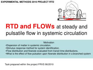
HYDRAULICS of steady and pulsatile flow in systemic circulation

1. 1 1 0 2 HYDRAULICS of steady and pulsatile flow in systemic circulation Motivation Experimental techniques for measurement pressure and flowrate How to calculate flow resistances in a branched system? What is the ratio of viscous and inertial effects upon pressure field? What is the effect of flow pulsation upon flowrate distribution in a branched system Task prepared within the project FRVS 90/2010

2. Laboratory model of circulation Simulated part - pressure transducers

3. NODES of simulation model Y [m] Data file defines the coordinates x,y,z of all 29 nodes 19 18 16 28 15 17 27 14 22 20 29 7 9 12 24 25 21 6 8 26 5 10 11 13 4 3 pressure transducers 23 Center of branching 2 Pressure p prescribed, flowrate Q calculated n Pressure p and flowrate Q are calculated m Define only geometry of branching k 1 X [m] -0.4 -0.3 -0.2 -0.1 0 0.1 0.2 0.3 0.4 0.5 0.6 0.7 0.8

4. ELEMENTS of simulation model V5(14,16,15,27,d3,d4,d4) V6(17,18,19,28,d3,d4,d4) V7(20,22,21,29,d3,d4,d4) P6(7,17,d3) P5(9,14,d3) P7(6,20,d3) V3(8,9,10,25,d2,d3,d3) 25 V2(5,6,7,24,d2,d3,d3) P4(8,11,d3) P3(4,8,d2) P2(3,5,d2) V4(11,12,13,26,d3,d4,d4) V1(2,3,4,23,d1,d2,d2) Nodal indices Data files define connectivity of PIPES (2-node elements) DIVISION-WYE (3-node elements) P1(1,2,d1)

5. UNKNOWNS and EQUATIONS 2N-Nb = 2Mp+3Mv N – number of nodes (unknowns p,Q) Mp – number of pipe elements Nb – number of boundary nodes (fixed p or Q) Mv – number of division elements Each element pipe generates 2 equations Each element of branching generates 3 equations

6. EQUATIONS generated by PIPES x2,y2,z2 p2,Q2 d 1. Continuity equation Q1 = Q2 2. Energy balance (Bernoulli equation) x1,y1,z1 p1,Q1 [J/kg] Potential energy (gravity) Pressure energy Inertia-pulsatile flow Irreversibly lost energy (dissipated to heat by viscous forces) Hagenbach factor describing losses related to velocity profile development at inlet of pipe Hagen-Poisseuile viscous losses corresponding to fully developed parabolic velocity profile t is constant viscosity at laminar flows, and almost linear function of flowrate in turbulent flows.

7. x2,y2,z2 p2,Q2 x3,y3,z3 p3,Q3 d1 x4,y4,z4 x1,y1,z1 p1,Q1 EQUATIONS generated by WYES 1. Continuity equation Q1 = Q2+Q3 2. Bernoulli equation between 1-2 3. Bernoulli equation between 1-3 Potential energy (gravity) Inertia-pulsatile flow Kinetic energy V=Q/cross section Pressure energy lost energy (viscous forces)

8. x2,y2,z2 p2,Q2 x3,y3,z3 p3,Q3 d1 x4,y4,z4 x1,y1,z1 p1,Q1 Resistance coefficients in WYES E.Fried, E.I.Idelcik: Flow resistance, a design guide for engineers E.I.Idelcik: Handbook of hydraulic resistances Rewritten in terms of flowrates and adding Hagen Poiseuille loses Hagen-Poisseuile viscous losses corresponding to fully developed parabolic velocity profile PROBLEMS: 1. Explain why the resistance coefficient ς must be infinite when Re  0 2. Coefficients in previous correlations are not reliable. Try to identify the effect of k parameter to results of your experiments simulation.

9. Simulation in MATLAB MATLAB M-files available at http: mainpq.m Input data files: xyz.txt x y z cb.txt i pq (boundary conditions i-node, +pressure, -flowrate as parameter pq) cp.txt i j d (pipe-indices of nodes and diameter) cv.txt i j k l d1 d2 d3(wye-indices of nodes and diameters) TASK: 1. Modify input files according to parameters of your experiment 2. Compare calculated and measured pressures 3. Evaluate dissipated power [W] in straight sections and in branching

10. Experiments: UVP flowrate Ultrasound Doppler effect for measurement velocity profiles • Piezotransducer is transmitter as well as receiver of US pressure waves operating at frequency 4 or 8 MHz. • Short pulse of few (10) US waves is transmitted (repetition frequency 244Hz and more) and crystal starts listening received frequency reflected from particles in fluid. • Time delay of sampling (flight time) is directly proportional to the distance between the transducer and the reflecting particle moving with the same velocity as liquid. • Received frequency differs from the transmitted frequency by Doppler shift Δf, that is proportional to the component of particle velocity in the direction of transducer axis. http://biomechanika.cz PROBLEMS: • What is spatial resolution of velocity, knowing speed of sound in water (1400 m/s) and sampling frequency 8 MHz ? • Calculate flowrate in a circular pipe from recorded velocity profile (given angle )

11. Experiments: pressure Δp • Pressure transducers CRESTO have silicon membrane with integrated strain gauges and amplifier. Pressure range 0-20 kPa. Feeding DC 5V, output also 5V, linear characteristics. • Flowrate can evaluated from two pressures measured at a straight section of circular pipe. In laminar flow regime the relationship between flowrate and pressure difference is Hagen-Poiseuille law. http://biomechanika.cz PROBLEMS: • Pressure differences are sometimes very small. Design experimental technique using water column in a glass tube. What is the pressure resolution in this case? • Estimate stabilization length for development of velocity profile (L/D=0.05Re)

12. LABORATORY REPORT • Front page: Title, authors, date • Content, list of symbols • Introduction, aims of project, references • Description of experimental setup • Experiments at different flowrates (laminar and turbulent flow regime). • Evaluate flowrate from recorded pressure drop. Check Re and flow regime. • Evaluate flowrate from velocity profiles recorded by UVP monitor. • Simulation (steady state). Modify input files and M-files according to measured flowrates and pressures. Compare measured and calculated pressures. Optimise parameters of hydraulic resistance correlation. • Adjust flowrate pulsation. • Evaluate effect of pulsation frequency upon radial velocity profiles using UVP monitors. Compare velocity profiles with analytical solution (Womersley 1955) • Conclusion (identify interesting results and problems encountered)