Download
1 / 29
290 likes | 416 Views
RD 51 Test beam. Large GEM testing. List of scans. Large GEM scans. N. Internal: A , D, E, H, I, L, M, O, P External border: F, N Junction zone: B , C, G. M. I. F. P. L. O. E. H. D. A. G. C. B. Pad dimensions: 7mm*3.5mm (smallest) to 35mm*17.5mm (biggest).

E N D
RD 51 Test beam Large GEM testing
Large GEM scans N Internal: A, D, E, H, I, L, M, O, P External border: F, N Junction zone: B, C, G M I F P L O E H D A G C B Pad dimensions: 7mm*3.5mm (smallest) to 35mm*17.5mm (biggest)
Large GEM gain curve N.B.: The low-gain part of the "right" curve is offset by incorrect zeroing of the nA-meter, at higher gain this becomes insignificant.
HV scan – point Pruns 21-108 – best efficiency over latencies = 13, 14, 15 clk; MSPL=4clk
HV scan – point Aruns 337-554 – best efficiency over latencies = 13, 14, 15, 16clk
Threshold scan – point Pruns 269-336 – latency = 14clk, MSPL = 4clk
Threshold scan – point Aruns 555-621 – latency = 14clk; MSPL = 4clk
Comparison: big pad VS small pad Big pad Small pad The smaller pad seems more efficient. This might be due to our efficiency-computing algorithm: we use to set a maximum residual of the hit on the large GEM with respect to the projecton of the track. We will investigate further on this effect.
Fine treshold scan – point Aruns 622-641 – I = 834uA (-5.00kV); lat = 14clk; MSPL = 4clk At low thresholds, the effect of the noise invalidates our efficiency measurements. To avoit this, the majority of our data takings were run at Th <= -40 DAC steps.
MSPL scan – point Pruns 109-268 – I = 859 uA (HV = -5.15kV) At Th=40 we have noise in the measurements, which intensity rises as we lenghten the monostable pulse. Thresholds are negative
Variable intensity hadrons – HV scanruns 653-693 – best efficiency over latencies = 14, 15clk; MSPL = 4clk We could not take more points, but it’s visible that the chamber reaches the plateau at lower HV than it does with leptons. We will investigate further on this behaviour.
Pad position scanruns 694-773 We will compare these data with the positions of the spacers on the chamber. we had some dead pad near pt M
Gas mixture changed fromAr-CO2 70/30to Ar-CF4 60/40 Testing the new gain / speed values
Minor latency scanruns 774-776 – I = 876uA (-5.25kV); th = -60steps; MSPL = 4clk We probably made some mistake in selecting the right working point and could not take more runs, so we miss the HV response of the large GEM with this Ar/CF4 60/40 gas mixture.
Gas mixture changed from Ar-CF4 60/40 to Ar-CF4-CO2 60/20/20 Testing the new gain / speed values
HV scanruns 857-869 – best efficiency over lat = 14, 15, 16clk; th = -60steps; MSPL=4clk We did not reach the plateau, but we did not want to go too high with the HV. The large GEM’s efficiency becomes high at higher HV than it does with the Ar/CO2 70/30 gas mixture. Here is a comparison of the two HV curves.
MSPL scan at HV = -5.30, -5.35kVruns 867-920 – I = 883, 892uA (-5.30, -5.35kV); th = -60steps With this mixture we have a better response, using MSPL = 1clk and MSPL = 2clk, than we have with Ar/CO2 70/30. 883uA scan 892uA scan
Gas mixture comparisonMSPL = 2clk; Ar/CO2 70/30 vs Ar/CO2/CF4 60/20/20 The signal is faster with Ar/CO2/CF4 60/20/20 gas mixture: it starts at latency = 18clk, and the peak reached is higher. Then, the chamber responce seems faster. We will investigate further on this point: these two scans were run at different gain values.
CMS Timing GEM scansGas mixture used: Ar/CF4 60/40 Working points:
Working point scan (Eff. VS Gain)runs 777-794 – Ed = 2kV/cm; Et1, Et2, Ei = 3kV/cm; th -20, lat 15-16-17, MSPL 4 Working point 7 was reached later and was not included in this HV scan.
Drift field scanruns 795-807 – E t1, Et2, Ei = 3kV/cm; th -20, lat 16, wrk points 4-6 At working point 6 the gain was too high to notice the variations.
Induction field scanruns 808-816 – Ed = 2kV/cm; Et1, Et2 = 3kV/cm; th -20, lat 16, MSPL 4, wrk pt4
MSPL scanruns 817-856 – Ed = 2kV/cm; Et1, Et2 = 3kV/cm; Ei = 4.5kV/cm; th -20steps, wrk pt 7 With this gas mixture the signal is faster than it is with Ar/CO2 70/30 mixture. At MSPL=1clk and MSPL=2clk the efficiency is already high.
Trackers – Preliminary threshold scanruns 0-15 – latencies = 14, 15clk; MSPL = 4clk • Efficiency was roughly computed as the number of times we had zero clusters on the chamber, in correspondance with a trigger signal, among the total number of events triggered by the scintillators. We still have to analyse the tracker’s response in HV, latency, and threshold.
Ar/CO2/CF4 60/20/20 specificationsdrift velocity, Townsend and attachment coefficients