Download
1 / 12
120 likes | 280 Views
Radial-Basis Function Networks (5.4 ~ 5.5) CS679 Lecture Note Compiled by Sang-eun, Bak AILAB.,CSD.,KAIST 99. 4. 19. Ill Posed Problme (1). Pitfall of strict interpolation Poor Generalization to new data - Overfitting “Hypersurface Reconstruction” Direct VS. Inverse Problem

E N D
Radial-Basis Function Networks (5.4 ~ 5.5) CS679 Lecture Note Compiled by Sang-eun, Bak AILAB.,CSD.,KAIST 99. 4. 19
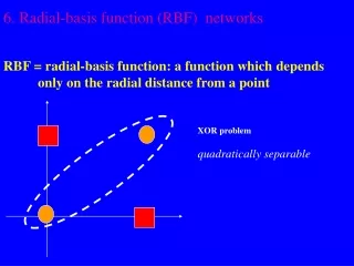
Ill Posed Problme (1) • Pitfall of strict interpolation • Poor Generalization to new data - Overfitting • “Hypersurface Reconstruction” • Direct VS. Inverse Problem • Well-posed or Ill-posed Problem • problem of reconstruction a mapping is “well-posed” if it satisfies ; • Existence • Uniqueness • Continuity • Otherwise, the problem is “Ill-posed” • meaning : Small information for desired output
Ill Posed Problem (2) • Hypersurface Reconstruction is Ill-posed Inverse Problem • Exist : no distinct output for every input • Uniqueness : small information for using I/O mapping uniquely • Noise and imprecision adds uncertainty for I/O mapping • may generate output over specific range : Violating Continuity • To overcome above problem, “Prior Information” must be needed! • Information about “I/O mappting”
Regularization (1) • Basic Idea • stabilize the solution by means of some auxiliary nonnegative functional that embeds prior information about the solution • prior information involves assumption “I/O mappting ftn. Is smooth” • In that sense, similar inputs correspond to similar outputs • Basic extention • Let : Input signal : Desired signal : • assumptions • output : one-dimensional • approximating ftn. be denoted by • Define • Standard Error Term : Denote • - error of sample data
Regularization (2) • Regularization Term : Denote • D is linear differential operator (including prior information about solution - I/O mapping) • also referred as a stabilizer • Tikhonov functional : “minimized value” • : The minimizer of • ramda : positive real number (regularization parameter) • indicator of sufficiency of given data set that specify the sol. • At case , problem is unconstrained ( is completely determined from the examples) • At case , prior smoothness constraint imposed by D is by itself sufficient to specify the sol. (example is unreliable)
Regularization (3) • In real world problem, so both sample data and prior information contribute to the solution. • Thus, represents a model complexity-penaly function and final sol. Is influenced by and parameter ramda
Frechet Differential of the Tikhonov Functional • Frechet Differential for Tinkhonov functional • may be interpreted as the best local linear approximation • defined such: • To solve minimizing problem, such condition is needed • After some steps of equations, each of terms result in such: • where • is inner product in Hilbert Space (Complete Inner Product Space)
Euler-Lagrange Equation • : adjoint operator (u(x) and v(x) are differentiable and satisfy proper boundary conditions) where • Applying this to the equation (3) • let u(x) = DF(x) and Dv(x) = Dh(x), then • Rewrite Equ. (1) with Equ. (2) and (3) : • is zero for every h(x) iff • equivalently • Equ. (5) is Euler-Lagrange equation; necessary condition for Tinkhonov functional to have an extremum at
Sol. to the Regularization Problem • For Green Ftn. (In detail, see P. 271) , a given differential operator L, and a continuous ftn of equ. is a sol. of diff. equ. • Let and then sol. described above will be changed : • Using sifting property of Dirac delta ftn., finally we get : • xi is center of expansion and weights represent the coefficients • The final sol. is linear weighted sum of basis for this subspace. - G(x,xi)
Determination of coefficient • Let , , and • then Equ. (6) will be such : and • Eliminating , , so • (for more detail version of invertible problem, See page 274)
Conclusion • The solution of regularization is • This equ. states following: • The regularization approach is equivalent to the expansion of the sol. in terms of a set of Green’s ftn., specified by D and associated boundary conditions. • # of Green’s ftn = # of examples user in the training process • If D is translationally and rotationally invariant, G(x, xi) will depend on the Euclidean norm of the difference vector : • Under these condition, Green’s ftn. must be a radial-basis ftn, then solution takes special form , which construct a linear ftn space with Euclidean distance measure
Multivariate Gaussian Functions • An example of Equ. (7) is Multivariate Gaussian Ftn, defined • xi : center of the ftn, : width of ftn. • Expansion in page 276 shows that multivariate gaussian ftn is a case of equ (7) • So, the regularized solution takes the form of a linear superposition as follows: • Each Gaussian member are assigned different variances. To simplify matters, same variance is often imposed on F(x). • Even though some limitation exist, RBF networks are still universal approximators