Download
1 / 10
100 likes | 471 Views
Self Organizing Maps. Self Organizing Maps. This presentation is based on: http://www.ai-junkie.com/ann/som/som1.html SOM’s are invented by Teuvo Kohonen. They represent multidimensional data in much lower dimensional spaces - usually two dimensions.

E N D
Self Organizing Maps • This presentation is based on: http://www.ai-junkie.com/ann/som/som1.html • SOM’s are invented by Teuvo Kohonen. • They represent multidimensional data in much lower dimensional spaces - usually two dimensions. • Common example is the mapping of colors from their three dimensional components - red, green and blue, into two dimensions. • 8 colors on the right have been presented as 3D vectors and the system has learnt to represent them in the 2D space. • In addition to clustering the colors into distinct regions, regions of similar properties are usually found adjacent to each other.
Network Architecture • Data consists of vectors, V, of n dimensions: V1, V2, V3…Vn • Each node will contain a corresponding weight vector W, of n dimensions: W1, W2, W3...Wn.
Network Example • Each node in the 40-by-40 lattice has three weights, one for each element of the input vector: • red, green and blue. • Each node is represented by a rectangular cell when drawn to display.
Overview of the Algorithm Idea: Any new, previously unseen input vector presented to the network will stimulate nodes in the zone with similar weight vectors. • Each node's weights are initialized. • A vector is chosen at random from the set of training data and presented to the lattice. • Every node is examined to calculate which one's weights are most like the input vector. The winning node is commonly known as the Best Matching Unit (BMU). • The radius of the neighborhood of the BMU is now calculated. This is a value that starts large, typically set to the 'radius' of the lattice, but diminishes each time-step. Any nodes found within this radius are deemed to be inside the BMU's neighborhood. • Each neighboring node's (the nodes found in step 4) weights are adjusted to make them more like the input vector. The closer a node is to the BMU, the more its weights get altered. • Repeat step 2 for N iterations.
Area of the neighborhood shrinks over time by shrinking the radius of the neighborhood over time For this use the exponential decay function: 0 is the width of the lattice at time t0 is a constant t is the iteration number Details Initializing the Weights • Set to small standardized random values 0 < w < 1 Calculating the Best Matching Unit • Use some distance Determining the Best Matching Unit's Local Neighborhood
Details Over time the neighborhood will shrink to the size of just one node... the BMU
Details Adjusting the Weights • Every node within the BMU's neighborhood (including the BMU) has its weight vector adjusted according to the following equation: • where t represents the time-step and L is a small variable called the learning rate, which decreases with time. • The decay of the learning rate is calculated each iteration using the following equation:
Details • Also, the effect of learning should be proportional to the distance a node is from the BMU.
Applications • SOM’s are commonly used as visualization aids. • They can make it easy to see relationships between vast amounts of data.