Feature descriptors and matching

1. Feature descriptors and matching

2. Feature detection and description • Harris corner detection gives: • Location of each detected corner • Orientation of the corner (given by xmax) • Scale of the corner (the image scale which gives the maximum response at this location) • Want feature descriptor that is • Invariant to photometric transformations, translation, rotation, scaling • Discriminative • P

3. Multiscale Oriented PatcheS descriptor • Describe a corner by the patch around that pixel • Scale invariance by using scale identified by corner detector • Rotation invariance by using orientation identified by corner detector • Photometric invariance by subtracting mean and dividing by standard deviation

4. Multiscale Oriented PatcheS descriptor • Take 40x40 square window around detected feature at the right scale • Scale to 1/5 size (using prefiltering) • Rotate to horizontal • Sample 8x8 square window centered at feature • Intensity normalize the window by subtracting the mean, dividing by the standard deviation in the window 40 pixels 8 pixels CSE 576: Computer Vision Adapted from slide by Matthew Brown

5. MOPS

6. Detour: Image transformations • What does it mean to rotate a patch? • Each pixel has coordinates (x,y) • Rotation represented by a matrix R • Pixel’s new coordinates: • I’(x’,y’) = I(x,y)

7. Detour: Image transformations • What if destination pixel is fractional? • Flip computation: for every destination pixel figure out source pixel • Use interpolation if source location is fractional • I’(x’, y’) = I(x,y)

8. Multiscale Oriented PatcheS descriptor Take 40x40 square window around detected feature • Scale to 1/5 size (using prefiltering) • Rotate to horizontal • Sample 8x8 square window centered at feature • Intensity normalize the window by subtracting the mean, dividing by the standard deviation in the window 40 pixels 8 pixels CSE 576: Computer Vision Adapted from slide by Matthew Brown

9. MOPS descriptor • You can combine transformations together to get the final transformation x T = ? y

10. Translate x y T = MT1

11. Rotate x y T = MRMT1

12. Scale x y T = MSMRMT1

13. Translate x y T = MT2MSMRMT1

14. Crop x y

15. Color and Lighting • Have invariance to additive and multiplicative changes to intensity • But what about more sophisticated changes to intensity?

16. Normal discontinuity Better representation than color: Edges Depth Discontinuity Albedo Edge Shadow

17. Out-of-plane rotation • Invariant to translation and rotation • But what about more sophisticated geometric transformations Out-of-plane rotation

18. Towards a better feature descriptor • Match pattern of edges • Edge orientation – clue to shape • Invariant to almost all photometric transformations • Be resilient to small deformations • Deformations might move pixels around, but slightly • Deformations might change edge orientations, but slightly

19. Invariance to deformation • Precise edge orientations are not resilient to out-of-plane rotations and deformations • But we can quantize edge orientation: only record rough orientation 37 42 Between 30 and 45

20. Invariance to deformation

21. Invariance to deformation • Deformation can also move pixels around • Again, instead of precise location of each pixel, only want to record rough location • Divide patch into a grid of cells • Record counts of each orientation in each cell: orientation histograms Orientation histogram

22. p 2 0 Rotation Invariance by Orientation Normalization [Lowe, SIFT, 1999] • Compute orientation histogram • Select dominant orientation (mode of the histogram; alternative to eigenvector of second moment matrix) • Normalize: rotate to fixed orientation T. Tuytelaars, B. Leibe

23. The SIFT descriptor SIFT – Lowe IJCV 2004

24. Scale Invariant Feature Transform • Basic idea: • DoG for scale-space feature detection • Take 16x16 square window around detected feature • Compute gradient orientation for each pixel • Throw out weak edges (threshold gradient magnitude) • Create histogram of surviving edge orientations angle histogram 2 0 Adapted from slide by David Lowe

25. SIFT descriptor • Create histogram • Divide the 16x16 window into a 4x4 grid of cells (2x2 case shown below) • Compute an orientation histogram for each cell • 16 cells * 8 orientations = 128 dimensional descriptor Adapted from slide by David Lowe

26. SIFT vector formation • Computed on rotated and scaled version of window according to computed orientation & scale • resample the window • Based on gradients weighted by a Gaussian

27. Ensure smoothness • Trilinear interpolation • a given gradient contributes to 8 bins: 4 in space times 2 in orientation

28. Reduce effect of illumination • 128-dim vector normalized to 1 • Threshold gradient magnitudes to avoid excessive influence of high gradients • after normalization, clamp gradients >0.2 • renormalize

29. Properties of SIFT Extraordinarily robust matching technique • Can handle changes in viewpoint • Up to about 60 degree out of plane rotation • Can handle significant changes in illumination • Sometimes even day vs. night (below) • Fast and efficient—can run in real time • Lots of code available: http://people.csail.mit.edu/albert/ladypack/wiki/index.php/Known_implementations_of_SIFT

30. Summary • Keypoint detection: repeatable and distinctive • Corners, blobs, stable regions • Harris, DoG • Descriptors: robust and selective • spatial histograms of orientation • SIFT and variants are typically good for stitching and recognition • But, need not stick to one

31. Which features match?

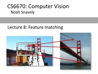
32. Feature matching Given a feature in I1, how to find the best match in I2? • Define distance function that compares two descriptors • Test all the features in I2, find the one with min distance

33. Feature distance How to define the difference between two features f1, f2? • Simple approach: L2 distance, ||f1 - f2 || • can give good scores to ambiguous (incorrect) matches f1 f2 I1 I2

34. Feature distance • How to define the difference between two features f1, f2? • Better approach: ratio distance = ||f1 - f2 || / || f1 - f2’ || • f2 is best SSD match to f1 in I2 • f2’ is 2nd best SSD match to f1 in I2 • gives large values for ambiguous matches f1 f2' f2 I1 I2