Download

1 / 22
220 likes | 357 Views
Chapter 5 Some Applications of Consumer Demand, and Welfare Analysis. Price Sensitivity of Demand. Elasticity of demand Percentage change in demand F rom a given percentage change in price. Price-Elasticity Demand Curves. Elastic demand, | ξ |>1 1% change in price

E N D
Chapter 5 Some Applications of ConsumerDemand, and Welfare Analysis
Price Sensitivity of Demand • Elasticity of demand • Percentage change in demand • From a given percentage change in price
Price-Elasticity Demand Curves • Elastic demand, |ξ|>1 • 1% change in price • >1% change in quantity demanded • Inelastic demand, |ξ|<1 • 1% change in price • <1% change in quantity demanded • Unit elastic demand, |ξ|=1 • 1% change in price • =1% change in quantity demanded
Elasticity along a linear demand curve Price μ Pmax q= a-b.p |ξ|>1 |ξ|=1 P1 |ξ|<1 0 Quantity A
Price-Elasticity Demand Curves • Perfectly inelastic demand curve • Perfectly vertical demand curve • Zero quantity response to a price change • Perfectly elastic demand curve • Horizontal demand curve • Price > p • Quantity = 0 • Price = p • Any quantity
Perfectly elastic & perfectly inelastic demand curves Price Price (a) (b) D D Perfectly inelastic demand curve. With zero elasticity, the quantity demanded is constant as prices change. Perfectly elastic demand curve. With infinite elasticity, the quantity demanded would be infinite for any price below p and zero for any price above p. 0 0 Quantity Quantity
Properties of Demand Functions • Price and income multiplication by the same factor leaves demand unaffected • “No money illusion property”
1. No Money Illusion Property Good 2 (x 2) f e B’ Multiplying all prices by the same factor shifts the budget line from BB’ to B’”B”. Multiplying prices and the agent’s income by the same factor has no effect on the budget line. B’” B” B 0 Good 1 (x 1)
2. Ordinal utility property Good 2 (x 2) e B Regardless of the utility numbers assigned to the three indifference curves, the agent maximizes utility by choosing point e. Thus demand is unaffected 120(8) 100(5) 90(3) B’ 0 Good 1 (x 1)
From Individual to Market Demand • Market demand curve • Aggregate of individual demand curves • Horizontally add up individual demand curves
Market demand from individual demand (d) (c) (b) (a) Aggregate demand Person k Person j Person i Price Price Price Price P1 P2 Dk Dj D Di 27 63 12 30 10 20 5 13 Quantity Quantity Quantity Quantity The market demand curve D is the horizontal summation of the individual demand curves Di , Dj , and Dk .
Welfare Measures • The welfare effects of price increase can be assessed using • Demand curve: • Loss in consumer surplus • Consumer choice model: • Price compensating variation
1. Consumer Surplus Consumer surplus • Net gain to consumers measured as the difference between the willingness to pay and the amount actually paid
1. Consumer Surplus Price Consumer surplus. The area under the demand curve and above the price measures the agent’s total willingness to pay for the quantity of the good she is consuming minus the amount she must pay. 33.3 CS 10 70 0 Quantity of cocaine demanded 100
Measures of Consumer Gain/ Loss • Loss of consumer surplus • Difference between • consumer surplus for price p • consumer surplus for price p+∆p
Change in consumer surplus Price a p+∆p p 0 Good 1 (x 1) When the price increases, the change in the area under the demand curve and above the price measures the welfare loss caused by the price change.
2. Price-compensating variation in income • Price-compensating variation in income measures the compensation needed due to an increase in price • To understand the price-compensating variation in income we first introduce the expenditure function • Expenditure function • Minimum income/expenditure amount (E) • To achieve a predetermined utility (u) • At given prices (p1,p2) • E=E(p1,p2,u)
The Expenditure Function • The problem • The Lagrangian
Derivation of an Expenditure function Good 2 (x 2) Suppose p1=$0.5 and P2=$1, What is the minimum level of income needed to bring the consumer to a utility level of u*? f e 17 15 7 I1(u*) B1 10 20 0 Good 1 (x 1) B2 B3
Measures of Consumer Gain/ Loss • Price-compensating variation in income • Additional income given to consumer • After price change • Same utility (before price change)
Price-compensating variation in income • Good 2 Suppose p1=$1 and P2=$1. If P2 increases to $2, How much extra income is needed to compensate the consumer? Price -compensating variation (in income) f e d B Z I1 I2 p 0 Good 1 (x 1) B’ B” ZB is the amount of income that must be given to the agent after the price increase in order to restore him to I1, the indifference curve he was on before the price change
Price-Compensating Variations andExpenditure Functions • Prices: p1, p2 • Utility level: u* • Expenditure: E=E(p1,p2,u*) • Increase in p1 to p1+ϵ • Expenditure: E’=E(p1+ϵ,p2,u*) • Price-compensating variation = E’-E= = E(p1+ϵ,p2,u*) - E(p1,p2,u*)