Download
1 / 21
250 likes | 662 Views
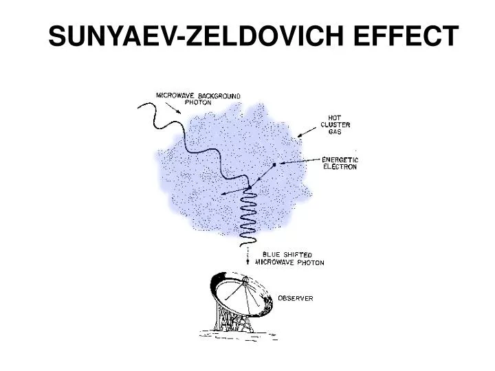
SUNYAEV-ZELDOVICH EFFECT. OUTLINE. What is SZE What Can we learn from SZE SZE Cluster Surveys Experimental Issues SZ Surveys are coming: What do we do?. INTRODUCTION. Inverse Compton Scattering of CMB photons. Decrement in intensity below SZ null (218 GHz), increment above

E N D
OUTLINE • What is SZE • What Can we learn from SZE • SZE Cluster Surveys • Experimental Issues • SZ Surveys are coming: What do we do?
INTRODUCTION • Inverse Compton Scattering of CMB photons. • Decrement in intensity below SZ null (218 GHz), increment above • Small spectral distortion of CMB of order ~1 mk. • Independent of redshift.
kSZ Effect The Doppler effect of line of sight cluster velocity -> observed shift of the CMB spectrum. In the nonrelativistic limit, the spectral signature of the kinetic SZE is a pure thermal distortion of magnitude of the CMB signal:
SZE FOR ASTROPHYSICS Cluster physics – measure integrated pressure Peculiar velocities at high z Cluster gas mass fraction, ΩM – clean measure of baryon gas mass Hubble constant, H(z) – combined with x-ray DA(z) Cluster surveys: – exploit redshift independence – constrain ΩM , ΩΛ σ8, w, w(t)… S
Cluster gas mass fraction, ΩM Since clusters collapse from large volumes of order 1000 Mpc3, the ratio of baryons to dark matter should be a reasonable approximation to the mix in the universe as a whole. Isothermal b model Constrain b and rc with SZE, integrate->total gas mass. Total mass of the cluster can be estimated from X-ray or lensing measurements. Grego et. al.,2001
Hubble constant, H(z) 33 SZ distances vs. redshift Ho = 63 3 km/s/Mpc for M = 0.3 and = 0.7, fitting all SZE distances
Constraining Dark Energy The observed cluster red-shift distribution in a survey is the co-moving volume per unit red-shift and solid angle dV/dzdW times the co-moving density of clusters ncl with masses above the survey detection limit Mlim. ~1/H(z) *mass function Majumdar,2004
CLUSTER SURVEYS WITH SZE • Create cluster catalogs independent (almost) of cosmology and redshift. • Trace structure formation from z~2 or 3 to present day. • Sample to study individual clusters to study cluster physics. Cluster Abundance Number density of clusters as a function of mass and redshift
Comoving volume element (left) and comoving number density (center) for two cosmologies, (ΩM, ΩΛ)=(0.3, 0.7) (solid ) and (0.5, 0.5) (dashed). (Middle) The normalization of the matter power spectrum was taken to be σ8=0.9 and the Press-Schechter mass function was assumed. The lower set of lines in the middle panel correspond to clusters with mass greater than 1015h−1Msun while the upper lines correspond to clusters with mass greater than 1014h−1Msun.
Mass Limits of Observability (1+z)4 enhancement compared to usual flux limit. z> 1, DA is slowly varying, Te is higher =>limiting mass of an SZ survey gently declines S Deep Surveys~10 clusters per square degree Less Deep Surveys (all sky Plank Survey) ~ 1 cluster every few square degree.
Experimental Challenge • Small signal • Must make differential measurements – Synchronous offsets • Contaminations – Radio Point Sources (synchrotron) – Point sources in mm/submm (Galactic and Extragalactic dust) – Primary anisotropies of the CMB .
SZE and PRIMARY CMB ANISOTROPY Arc minute anisotropy dominated by diffuse SZE except at λ’s near SZE null SZE requires small beam and/or multi-frequency observations
Point Source Removal Point source removed low resolution Point source removed high resolution Point source
SZ Surveys are coming: What should we do Simulations to study survey selection function and observable uncertainties Plot of the matched filter noise Y as a function of filter scale qc (core radius of a cluster matched to the filter) for different surveys, as labeled. The filter noise is generated by primary CMB anisotropy and instrumental noise. Clusters lying above the curve of a particular experiment have S/N > 1. Bartlett,2006
SZ Surveys are coming: What should we do Integrated source counts at S/N > 5 for each survey are shown , along with the simulation input counts (curve labeled “mass function”). Catalog completeness percentage (ratio of the experimental curve to the input mass function counts) is given in the inset.The important point is that the surveys are not flux limited, and are significantly incomplete even at 5 times their point source sensitivities. Bartlett,2006
SZ Surveys are coming: What should we do Photometric recovery in terms of integrated Compton Y parameter for SPT (left) and AMI (right). Compton Y values (in arcmin2) recovered by the matched filter are plotted against the input Y values taken from the simulation catalog. Each point represents a single cluster detected at S/N > 5. The red dashed curve gives the equality line. For SPT the characteristic scatter at fixed Ytrue is 40%. Confusion with primary CMB anisotropy seriously compromises photometric recovery of the single frequency survey (chosen here as AMI). Multiple frequency observation or a follow up in X-ray is necessary Bartlett,2006
SUMMARY CLUSTERS ARE GREAT!!! SZE is COOL. However….