Download
1 / 18
190 likes | 492 Views
Regression and Correlation (and scatter plots). Outline. Making a Scatter plot Calculating the Regression Line The Correlation Alternative Procedures Further Considerations of Regressions and Correlations. Estimating the speed of a car. Four Steps. Regression Lines. Different types

E N D
Outline • Making a Scatter plot • Calculating the Regression Line • The Correlation • Alternative Procedures • Further Considerations of Regressions and Correlations
Regression Lines • Different types • Here, a straight line that gets close to most of points. • One way to define “close to most points” is by finding the line that minimizes the sum of the squared vertical distances from line to the points. Minimizing ∑ei2. • Called ordinary least squares (OLS) regression.
What is a straight line? • In mathematics: y = ax + b a is the slope b is the intercept • In statistics: yi = β0 + β1 xi + ei Subscripts show people have different values on variables Β0 is the intercept β1 is the slope ei are the residuals: the vertical distance between the line and the points.
Lots of calculations Estimate for β1 = 358.8/625.6 = 0.5735 Estimate for β0 = 14.4 - .5735(18.8) = 3.62.
SStotal = SSmodel + SSresidual • SStotal is 956.4 • SSresidual is 750.6 • SSmodel = SStotal - SSresidual = 956.4 – 750.6 = 205.8 • R2= SSmodel / SStotal = 205.8/956.4 = 0.22 • R2 = the proportion of variation accounted for by the model. • Square root of R2, R (or r), also useful.
Testing hypothesis R2 = 0 in the population • dfmodel = # variables in the model (here 1) • dferror = n - dfmodel – 1 (here 10 – 1 – 1 = 8) • MSSmodel = SSmodel /dfmodel (here 205.8/1 = 205.8) • MSSerror = SSerror /dferror (here 750.6/8 = 93.8) • F(dfmodel, dferror) = MSSmodel/MSSerror • F(1,8) = 205.8/93.8 = 2.19 • If computer doing the calculations, p = .18.
Pearson’s Correlation r Square root of R2, but keeping the sign. Ranges from -1 to 1, with negative associations having negative r values.
Testing if r = 0 in the population Also worth calculating confidence intervals (see text)
An Alternative Procedure: Spearman's rS • Rank the data, and then run Pearson’s • Some complications and variations if there are lots of ties. • Impact of univariate outliers (both those that increase the r and decrease it) r = .94 rS = .78 r = .76 rS = .74
Further Considerations • What we have discussed has been for straight lines. Look at scatter plots to see if other techniques for curves necessary. • Correlation does not imply causation (but it suggests that somewhere in the network of hypotheses that includes these two variables that there are causal relationships).