Download
1 / 66
710 likes | 922 Views
Finite Capacity Scheduling. 6.834J, 16.412J. Overview of Presentation. What is Finite Capacity Scheduling? Types of Scheduling Problems Background and History of Work Representation of Schedules Representation of Scheduling Problems Solution Algorithms Summary.

E N D
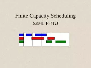
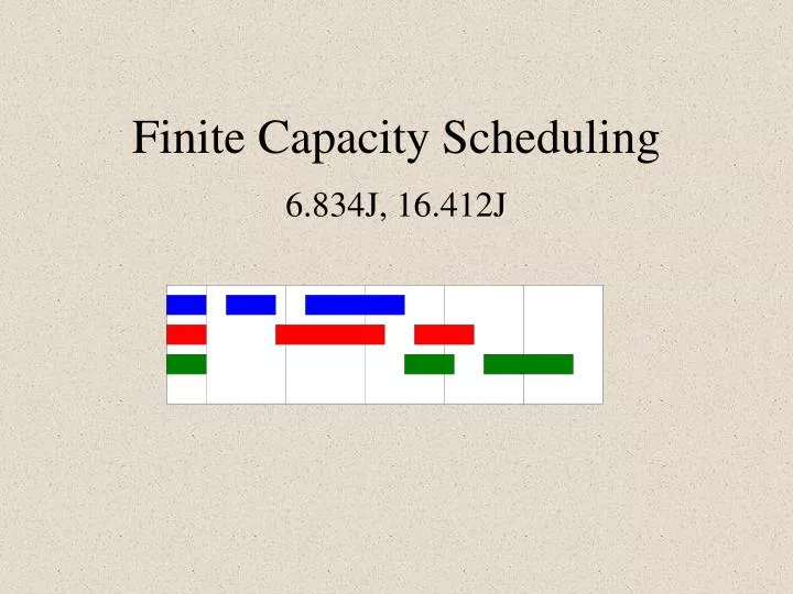
Finite Capacity Scheduling 6.834J, 16.412J
Overview of Presentation • What is Finite Capacity Scheduling? • Types of Scheduling Problems • Background and History of Work • Representation of Schedules • Representation of Scheduling Problems • Solution Algorithms • Summary
What is Finite Capacity Scheduling? • Informal and Partial Definitions • Determining the best sequence of tasks on a resource • Optimal assignment of limited resources to tasks to fulfill a set of orders • Elimination of factory bottlenecks • Formal Definition • The allocation of resources over time to perform a set of tasks • such that task precedence constraints and resource capacity constraints are not violated, and overall deadline goals are met to the best extent possible
Example Schedule • Gantt chart
Types of Scheduling Problems • Energy • Job Shop • Batch Process • Discrete Manufacturing • Servicing of Complex Equipment • Scheduling of a Unique Resource • Military Logistics
Energy Scheduling • Electrical utility generator scheduling to meet anticipated demand • Ex. – Utility with 3 Generators
Energy Scheduling (cont.) • Demand Profile
Energy Scheduling (cont.) • Best Schedule:
Let if generator i is on during time j, 0 otherwise be the energy generated by generator i during time j Cost can then be expressed as From the previous schedule, non-zero values of B and E are: So cost = 70 + 88 + 60 + 24 = 242
Constraints for this problem can be expressed as Where is demand at time j, and is the capacity of generator i. Note how this forces Eij to be 0 if Bij is. This, combined with the constraint that the B variables must be binary, and the previously defined cost function, yields an optimization problem with discrete and continuous constraints. Such problems are often solved by Mixed Integer Linear Programming algorithms (more on this later).
Variations on Problem • Suppose utility has 100 kwh energy storage device (battery that has no hourly or incremental cost) • Could run generator 2 during 1st hour to charge battery • Could then discharge battery to meet demand in 3rd hour • Eliminates need to use generator 3 • Suppose another consumer would like to buy energy • New consumer has their own demand profile • Utility must evaluate whether it is profitable to sell to this new customer • This is a function of base demand profile, consumer’s demand profile, generation costs, and what the new consumer is willing to pay • Suppose generator 3 has high hourly cost but low energy cost • It may make sense to run it and shut off generators 1 and 2
Variations on Problem – Co-generation • Co-generation introduces a new set of complex considerations • Ex. – Refinery that uses waste heat from process to make steam to generate electricity • Refinery may schedule production to simultaneously meet production goals and demand for electricity, thus maximizing profit • Two kinds of demand • Refinery’s main products (gasoline of various grades, etc.) • Electricity (demand profile as shown previously) • Also complicated by the fact that electricity prices vary based on demand, and on time of day • Contracts between factories, utilities, and customers can be extremely complicated
Job Shop Scheduling • Schedule n jobs on m machines • Each job requires processing on each machine in a particular order • This order differs from one job to another • Often formulated as constraint satisfaction problem with binary temporal constraints among the mn tasks • Eliminating bottleneck resources is an important goal
Batch Process Scheduling • Tasks have “size” that is a continuous and/or discrete function of the amount of material to be produced to fulfill an order • Task size can affect task duration, resource requirements • Resource utilization represented with a combination of discrete and continuous variables • Often, and important goal is to find ways to combine similar tasks into larger “batches” in order to minimize changeover costs
Example – Beer Production • After brewing and aging, beer must be filtered, prior to packaging.
Discrete Manufacturing Scheduling • Semiconductor • Auto assembly • Heavy equipment • Aircraft assembly • Electronic parts assembly
Discrete Manufacturing Scheduling (cont.) • Characteristics • Similar, in some ways, to job shop, and to batch process scheduling • Process plan instantiated based on order • Process plans for similar types of orders are similar • Fewer continuous variables and constraints • Task sizes are discrete functions of order • Ex. – a car needs 4 tires • Resource allocations are typically binary • Resource is utilized or not • Resources typically allocated to tasks for individual orders • Typically, no batching of tasks
Scheduling Service of Complex Equipment • Ex. – Space Shuttle Ground Processing • Approximately 40,000 hours of technician labor between flights.
Space Shuttle Service (cont.) • About 50% same for each flight. Rest is function of • payloads, • maintenance based on age of components • orbiter modifications • Very dynamic environment • Arrival date subject to change (and affected by weather) • Resource requirements – parts, supplies, people • State (configuration) of system being repaired is important • State constraints (requirements and effects), very important • Use of changeover tasks to get system into correct state
Scheduling of a Unique Resource • Ex. – Hubble Telescope
Scheduling of Hubble Telescope (cont.) • 10,000 to 30,000 observations scheduled per year • Primary resource constraint is available observing time • Affected by orbital position • Required orientation to keep sunlight on solar panels • Many constraints periodic • Disruptions • Targets of opportunity (new supernova) • Spacecraft anomalies • Changes in observing programs
Military Logistics • Transportation of troops and supplies • Resources to be scheduled are transport vessels and cargo planes • Groups of troops and supplies represent tasks • Resource capacity constraints significant • Deadline constraints significant • Precedence constraints significant • Equipment must be delivered in appropriate sequence
Background of Work on Scheduling(a representative, but not exhaustive list) • MRP (Material Requirements Planning), MRP II (1970’s) • Demand for end-products expanded into time-phased requirements for parts • Timing based on operation leadtimes • No accounting of resource loading • Schedules often un-realistic • Mark Fox, CMU, ISIS (1980’s) • Each order scheduled one at a time • Constructive approach, incrementally extends partial schedule solution until complete • Simple best-first search with backtracking • Formulation as CSP, hard and soft constraints, continuous and discrete • Some constraint propagation (forward chaining) capability
Background of Work on Scheduling (cont.) • Monte Zweben, NASA, Gerry (1990’s) • Iterative repair algorithm • Modifies complete schedule to repair constraints, or to make more optimal • Hill-climbing, search states are complete solutions • Pantelides, Imperial College (1990’s) • Chemical Process Scheduling • RTN, MILP algorithm • Discrete time formulation • Branch and bound, branch and cut
Areas of Work Related to Scheduling • Assignment Problem • Assign n tasks to n resources (no time rep.) • Specialized algorithm solves this efficiently • Transportation Problem • Transfer material between nodes in a graph • Traveling Salesman Problem • Resource “visits” n tasks (optimal sequencing of tasks on a resource) • Graph theory, flow networks (used in TSP) • Long-Range Planning • using Dynamic Programming • Combinatoric Optimization, CSP, A* search, MILP
Representation of Schedules • Task • Start time • Finish time • Duration • Resource assignments • Resource • Renewable (equipment for example) • Non-renewable (material or product, for example) • Useful to think of task as consuming one set of resources, and producing another set • For equipment, the task “consumes” the resource at the start time, and “produces” it (makes it available again) at the finish time.
Representation of Schedules (cont.) • Attributes of materials (non-renewable) resources - amount and state • Amount of flour, number of loaves of bread – related to task size • State – temperature of bread, freshness • Attributes of equipment (renewable) resources – state • Oven at input is clean (required state), oven at output is dirty (effect) • Cleaning oven is “changeover” task • Baker at output is tired (taking a knap might be changeover) • Attributes of tasks related to those of resources
Representation of Schedules:Discrete vs. Continuous Time Representations • Discrete • Scheduling horizon divided into discrete, equal intervals • Task start, finish times expressed in terms of these increments • Advantageous for certain scheduling algorithms • Easy to check for resource capacity violations • Disadvantage is that if fine time granularity over longer scheduling horizon is required, then many intervals • Problem size becomes un-manageable • Continuous • Task start, finish times expressed as real numbers • Smaller number of variables • Discrete event vs. discrete time • Disadvantage is that checking resource capacity violations is more complicated • Rules out use of certain scheduling algorithms
Representation of Scheduling Problems • Resource-Operation Network (RON) • Inspired by Imperial College RTN • Consists of Operations and Resource Requirements • Operation • Class of task • Duration may be constant, or may be function of other things • Other attributes (amount, type of material to be produced) • Resource Requirement • Renewable and non-renewable resources • Incorporates notion of state (of a material or a resource) • Task is an instantiation of an operation • Resource assignment is an instantiation of a resource requirement
Representation of Scheduling Problems (cont.) • - Note similarity to schedule representation • Attributes of operations and resource requirements similar • to attributes of tasks and resources
Representation of Scheduling Problems:Constraints • Resource requirements, Operations have attributes • Some general (like duration, start-time, etc.) • Some problem specific (state of a particular resource type) • Attributes can have discrete or continuous values • Combination of algebraic and logical constraints used to constrain values of attributes • Kneading.finish_time < Baking.start_time • Baking.OvenInput.Status = clean • Baking.Dough.amount = f(Baking.size) • RON architecture is general enough to support just about any kind of constraint (algebraic, logical, even functions) • However, there are a number of important basic types of constraints that are often used in scheduling
Representation of Scheduling Problems:Common Constraint Types • Constraints associated with resources • Resource utilization (how much of a resource a task needs) • Resource capacity (resource utilization should not exceed this) • Resource state • Task may require resource to be in particular state at beginning of task • Task may leave resource in particular state at end of task (effect) • Motivation for changeover tasks • Resource availability (calendar) • Resource (labor for example) may not be available on weekends • Constraints associated with tasks • Duration (may be constant, or may be function of task size) • Start, finish (related by duration) • Precedence (kneading before baking) • Usually not necessary when using RON formulation (falls out) • Due dates (ultimately, the reason for doing scheduling)
Resource Utilization Constraints • Operation usually determines amount of resource required, and amount produced • May be simple constant: • Baking.Oven_Input.amount = 1 (need one oven) • Baking.Oven_Output.amount = 1 (oven not consumed by process) • May be integer function of task size • Baking.Size = Baking.Break.Loaves (task size = number of loaves) • Baking.Flour.amount = 12 x Baking.Size • May be continuous function of task size • HoldingTank.level = 50 x Filtering.Size • May even be a complex, non-linear function • Lubricant.amount = f(Drilling.Size)
Resource Capacity Constraints • Resource utilization should not exceed maximum capacity for a resource • Resource utilization becomes function of time over scheduling horizon
Resource State Constraints • Constraint on state of input resource requirement • Analogous to requirement part of planning operation (Graphplan, etc.) • Baking.Oven_Input.status = clean • Constraint on state of output resource requirement • Analogous to effects part of planning operation • Baking.Oven_Output.status = dirty • Changeover operation used to restore resource to required state • Cleaning operation converts dirty oven to clean one • State requirements, changeover operations, often the key issue in generating good schedule • Reason: changeover operations take time (setup time) • Goal is often to minimize changeovers • This can be achieved by batching similar tasks • There is a limit to this, however, imposed by limits of inventory (resource capacity constraints)
Soft Constraints and Cost • It is often advantageous to think of scheduling as a constrained (or even un-constrained) optimization problem, rather than a constraint satisfaction problem • Analogous to notion of Lagrange multipliers in non-linear constrained optimization • Allow some constraints to be relaxed (make them soft) • However, relaxation has a cost penalty • Relaxation of deadline constraint results in lateness penalty • Relaxation of resource capacity constraint results in overtime pay requirement • Production costs usually directly associated with resource utilization • Thus, cost function is sum of • Resource utilization costs • Constraint relaxation penalties
Process Plan Instantiation • Instantiate tasks for process plan (operations) for each order • Ex. 3 orders for bread
Instantiated Tasks (Based on Process Plan) Also, Cleaning1, Cleaning2, and Cleaning3 (size not an issue for these)
Process Plan Instantiation (cont.) • Initial resource assignment based on resource requirements using very simple dispatch heuristics • Sequence tasks on resource based on order
Process Plan Instantiation (cont.) • This actually is not a bad schedule in some circumstances • Probably is a good schedule for this example • On the other hand, if the baker doesn’t care about freshness, and wants to take Tues. off • Batch orders together to improve efficiency • Requires inventory capacity • Refrigerated storage space • Tolerance to reduction in quality (quality is a state variable that decays over time)
Solution of Scheduling Problems • Unlike representation, which is relatively universal, solution algorithm is problem-dependent • Most real-world problems also require heuristics, specialized for the particular type of problem
Solution Algorithms • Dispatch Algorithms • MILP • Relation to A*, constructive constraint-based • Constructive Constraint-Based • Iterative Repair • Simulated Annealing • How A* heuristics can be used here (relaxation of deadline constraints) • Genetic Algorithms
Dispatch Algorithms • Process plan instantiated (as described previously) • Tasks put into queues, one for each order • (Preserves task precedence constraints)
Dispatch Algorithms (cont.) • Tasks released one at a time from queues • Assigned to first available resource • Which queue is popped depends on task priorities • Queue with highest priority task at top gets popped • Task priority based on variety of factors • Mainly order importance and urgency • Apex system is a dispatch system • Flight controller assistant, described by Rob Kochman
Dispatch Algorithms (cont.) • Advantages • Simple to implement • Can easily handle changing requirements by updating priorities • Disadvantages • When task is popped, it is assigned to first available resource • If none available, it just waits, and nothing further can be done • Thus, susceptible to bottlenecks • Doesn’t really set schedule times • Can’t guarantee when things will get done • No look-ahead, so no optimization • No capability for JIT • Tasks “shifted to the left”
Dispatch Algorithms (cont.) • However • Much, if not most, real-world scheduling is done in this way • Manual scheduling is often done in this way
MILP (Mixed Integer Linear Programming) • Used for energy scheduling • Chemical process scheduling • Pantelides, et. al., Imperial College • Sometimes used in discrete manufacturing • Pekny, Miller, Traveling Salesman Problems • For scheduling, requires discrete time formulation
MILP Basics • Constraints represented as linear equalities and inequalities • A is constant matrix, b is constant vector, x is vector of variables • X vector has lower and upper bounds • X consists of real and integer variables • Cost represented as weighted sum of x
MILP Basics • Energy scheduling example presented previously is an example of an MILP