Download
1 / 47
470 likes | 674 Views
Chapter 11: Storage and File Structure. Chapter 11: Storage and File Structure. Overview of Physical Storage Media Magnetic Disks RAID Tertiary Storage Storage Access File Organization Organization of Records in Files Data-Dictionary Storage. Classification of Physical Storage Media.

E N D
Chapter 11: Storage and File Structure • Overview of Physical Storage Media • Magnetic Disks • RAID • Tertiary Storage • Storage Access • File Organization • Organization of Records in Files • Data-Dictionary Storage
Classification of Physical Storage Media • Speed with which data can be accessed • Cost per unit of data • Reliability • data loss on power failure or system crash • physical failure of the storage device • Can differentiate storage into: • volatile storage: loses contents when power is switched off • non-volatile storage: • Contents persist even when power is switched off. • Includes secondary and tertiary storage, as well as battery backed up main-memory.
Physical Storage Media • Cache – fastest and most costly form of storage; volatile; managed by the computer system hardware. • Main memory: • fast access • generally too small (or too expensive) to store the entire database • capacities of up to a few Gigabytes widely used currently • Capacities have gone up and per-byte costs have decreased steadily and rapidly • Volatile — contents of main memory are usually lost if a power failure or system crash occurs.
Physical Storage Media (Cont.) • Flash memory • Data survives power failure • Data can be written at a location only once, but location can be erased and written to again • Can support only a limited number (10K – 1M) of write/erase cycles. • Erasing of memory has to be done to an entire bank of memory • Reads are roughly as fast as main memory • But writes are slow (few microseconds), erase is slower • Cost per unit of storage roughly similar to main memory • Widely used in embedded devices such as digital cameras • Is a type of EEPROM (Electrically Erasable Programmable Read-Only Memory)
Physical Storage Media (Cont.) • Magnetic-disk • Data is stored on spinning disk, and read/written magnetically • Primary medium for the long-term storage of data; typically stores entire database. • Data must be moved from disk to main memory for access, and written back for storage • Much slower access than main memory (more on this later) • direct-access – possible to read data on disk in any order, unlike magnetic tape • Capacities range up to roughly 400 GB currently • Much larger capacity and cost/byte than main memory/flash memory • Growing constantly and rapidly with technology improvements (factor of 2 to 3 every 2 years) • Survives power failures and system crashes • disk failure can destroy data, but is rare
Physical Storage Media (Cont.) • Optical storage • non-volatile, data is read optically from a spinning disk using a laser • CD-ROM (640 MB) and DVD (4.7 to 17 GB) most popular forms • Write-one, read-many (WORM) optical disks used for archival storage (CD-R, DVD-R, DVD+R) • Multiple write versions also available (CD-RW, DVD-RW, DVD+RW, and DVD-RAM) • Reads and writes are slower than with magnetic disk • Juke-box systems, with large numbers of removable disks, a few drives, and a mechanism for automatic loading/unloading of disks available for storing large volumes of data
Physical Storage Media (Cont.) • Tape storage • non-volatile, used primarily for backup (to recover from disk failure), and for archival data • sequential-access– much slower than disk • very high capacity (40 to 300 GB tapes available) • tape can be removed from drive storage costs much cheaper than disk, but drives are expensive • Tape jukeboxes available for storing massive amounts of data • hundreds of terabytes (1 terabyte = 1012 bytes) to even a petabyte (1 petabyte = 1015 bytes)
Storage Hierarchy (Cont.) • primary storage: Fastest media but volatile (cache, main memory). • secondary storage: next level in hierarchy, non-volatile, moderately fast access time • also called on-line storage • E.g. flash memory, magnetic disks • tertiary storage: lowest level in hierarchy, non-volatile, slow access time • also called off-line storage • E.g. magnetic tape, optical storage
Magnetic Hard Disk Mechanism NOTE: Diagram is schematic, and simplifies the structure of actual disk drives
Magnetic Disks • Read-write head • Positioned very close to the platter surface (almost touching it) • Reads or writes magnetically encoded information. • Surface of platter divided into circular tracks • Over 50K-100K tracks per platter on typical hard disks • Each track is divided into sectors. • A sector is the smallest unit of data that can be read or written. • Sector size typically 512 bytes • Typical sectors per track: 500 (on inner tracks) to 1000 (on outer tracks) • To read/write a sector • disk arm swings to position head on right track • platter spins continually; data is read/written as sector passes under head • Head-disk assemblies • multiple disk platters on a single spindle (1 to 5 usually) • one head per platter, mounted on a common arm.
Magnetic Disks (Cont.) • Earlier generation disks were susceptible to head-crashes • Surface of earlier generation disks had metal-oxide coatings which would disintegrate on head crash and damage all data on disk • Current generation disks are less susceptible to such disastrous failures, although individual sectors may get corrupted • Disk controller – interfaces between the computer system and the disk drive hardware. • accepts high-level commands to read or write a sector • initiates actions such as moving the disk arm to the right track and actually reading or writing the data • Computes and attaches checksums to each sector to verify that data is read back correctly • If data is corrupted, with very high probability stored checksum won’t match recomputed checksum • Ensures successful writing by reading back sector after writing it • Performs remapping of bad sectors
Disk Subsystem • Multiple disks connected to a computer system through a controller • Controllers functionality (checksum, bad sector remapping) often carried out by individual disks; reduces load on controller • Disk interface standards families • ATA (AT adaptor) range of standards [ATA: Adv Tech Attachment] • SATA (Serial ATA) - Parallel ATA • SCSI (Small Computer System Interconnect) range of standards • Several variants of each standard (different speeds and capabilities) • IDE – Integrated Drive Electronics
Performance Measures of Disks • Access time – the time it takes from when a read or write request is issued to when data transfer begins. Consists of: • Seek time – time it takes to reposition the arm over the correct track. • Average seek time is 1/3 if all tracks had the same number of sectors, and we ignore the time to start and stop arm movement • 4 to 10 milliseconds on typical disks • Rotational latency – time it takes for the sector to be accessed to appear under the head. • Average latency is 1/2 the time for a full rotation of the disk • 4 to 11 milliseconds on typical disks (5400 to 15000 r.p.m.) • Data-transfer rate– the rate at which data can be retrieved from or stored to the disk. • 25 to 100 MB per second max rate, lower for inner tracks
Performance Measures (Cont.) • Mean time to failure (MTTF) – the average time the disk is expected to run continuously without any failure. • Typically 3 to 5 years • Probability of failure of new disks is quite low, corresponding to a“theoretical MTTF” of 500,000 to 1,200,000 hours for a new disk • E.g., an MTTF of 1,200,000 hours for a new disk means that given 1000 relatively new disks, on an average one will fail every 1200 hours • MTTF decreases as disk ages
RAID • RAID: Redundant Arrays of Independent Disks • disk organization techniques that manage a large numbers of disks, providing a view of a single disk of • high capacity and high speed by using multiple disks in parallel, and • high reliability by storing data redundantly, so that data can be recovered even if a disk fails • Originally a cost-effective alternative to large, expensive disks • I in RAID originally stood for ``inexpensive’’ • Today RAIDs are used for their higher reliability and bandwidth. • The “I” is interpreted as independent
Improvement of Reliability via Redundancy • Redundancy – store extra information that can be used to rebuild information lost in a disk failure • E.g., Mirroring(or shadowing) • Duplicate every disk. Logical disk consists of two physical disks. • Every write is carried out on both disks • Reads can take place from either disk • If one disk in a pair fails, data still available in the other • Data loss would occur only if a disk fails, and its mirror disk also fails before the system is repaired • Probability of combined event is very small • Except for dependent failure modes such as fire or building collapse or electrical power surges • Mean time to data loss depends on mean time to failure, and mean time to repair
Improvement in Performance via Parallelism • Bit-level striping – split the bits of each byte across multiple disks • In an array of eight disks, write bit i of each byte to disk i. • Each access can read data at eight times the rate of a single disk. • But seek/access time worse than for a single disk • Bit level striping is not used much any more • Block-level striping– stripes blocks across multiple disks • Requests for different blocks can run in parallel if the blocks reside on different disks
RAID Levels • Schemes to provide redundancy at lower cost by using disk striping combined with parity bits • Different RAID organizations, or RAID levels, have differing cost, performance and reliability characteristics • RAID Level 0: Block striping; no mirroring or parity offered. • Used in high-performance applications where data lose is not critical. • RAID Level 1: Mirrored disks with block striping • Offers best write performance. • Popular for applications such as storing log files in a database system.
RAID Levels (Cont.) • RAID Level 2: Memory-Style Error-Correcting-Codes (ECC) with bit striping. • RAID Level 3: Bit-Interleaved Parity • a single parity bit is enough for both error correction and just detection • When writing data, corresponding parity bits must also be computed and written to a parity bit disk • Level 3 is as good as level 2, but is less expensive in the number of extra disks
RAID Levels (Cont.) • RAID Level 3 (Cont.) • Faster data transfer than with a single disk, but fewer I/Os per second since every disk has to participate in every I/O. • Subsumes Level 2 (provides all its benefits, at lower cost). • RAID Level 4: Block-Interleaved Parity; uses block-level striping like level 0, and keeps a parity block on a separate disk for corresponding blocks from N other disks. • When writing data block, corresponding block of parity bits must also be computed and written to parity disk • Data transfer rate is slower but multiple read access can proceed in parallel, thereby high overall i/o rate.
RAID Levels (Cont.) • RAID Level 4 (Cont.) • Provides higher I/O rates for independent block reads than Level 3 • block read goes to a single disk, so blocks stored on different disks can be read in parallel • Provides high transfer rates for reads of multiple blocks than no-striping • Before writing a block, parity data must be computed • Parity block becomes a bottleneck for independent block writes since every block write also writes to parity disk • Example: A single write requires 4 disk accesses – two to read the 2 old blocks, two to write the 2 blocks
RAID Levels (Cont.) • RAID Level 5: Block-Interleaved Distributed Parity; partitions data and parity among all N + 1 disks, rather than storing data in N disks and parity in 1 disk. • All disks can participate in satisfying read requests so Level 5 increases the total number of requests that can be met in a given amount of time.
RAID Levels (Cont.) • RAID Level 5 (Cont.) • Higher I/O rates than Level 4. • Block writes occur in parallel if the blocks and their parity blocks are on different disks. • Subsumes Level 4: provides same benefits, but avoids bottleneck of parity disk. • RAID Level 6: P+Q Redundancy scheme; similar to Level 5, but stores extra redundant information to guard against multiple disk failures. • Better reliability than Level 5 at a higher cost; not used as widely. • Instead of parity, Level 6 uses Error Correcting Codes • System can tolerate up to two failures.
Choice of RAID Level • Factors in choosing RAID level • Monetary cost • Performance: Number of I/O operations per second, and bandwidth during normal operation • Performance during failure • Performance during rebuild of failed disk • Including time taken to rebuild failed disk • RAID 0 is used only when data safety is not important • E.g. data can be recovered quickly from other sources • Level 2 and 4 never used since they are subsumed by 3 and 5 • Level 3 is not used anymore since bit-striping forces single block reads to access all disks, wasting disk arm movement, which block striping (level 5) avoids • Level 6 is rarely used since levels 1 and 5 offer adequate safety for almost all applications • So competition is between 1 and 5 only
Choice of RAID Level (Cont.) • Level 1 provides much better write performance than level 5 • Level 5 requires at least 2 block reads and 2 block writes to write a single block, whereas Level 1 only requires 2 block writes • Level 1 preferred for high update environments such as log disks • Level 1 had higher storage cost than level 5 • Disk storage capacities increasing rapidly (50%/year) whereas disk access speeds have improved at a much slower rate (x 3 in 10 years) • I/O requirements have increased greatly, e.g. for Web servers • When enough disks have been bought to satisfy required rate of I/O, they often have spare storage capacity • so there is often no extra monetary cost for Level 1! • Level 5 is preferred for applications with large amounts of data, where data are read frequently, and written rarely • Level 1 is preferred for all other applications
Hardware Issues • Software RAID: RAID implementations done entirely in software, with no special hardware support • Hardware RAID: RAID implementations with special hardware • Use non-volatile RAM to record writes that are being executed • Beware: power failure during write can result in corrupted disk • E.g. failure after writing one block but before writing the second in a mirrored system • Such corrupted data must be detected when power is restored • Recovery from corruption is similar to recovery from failed disk • NV-RAM helps to efficiently detect potentially corrupted blocks • Otherwise all blocks of disk must be read and compared with mirror/parity block
Hardware Issues (Cont.) • Hot swapping: replacement of disk while system is running, without power down • Supported by some hardware RAID systems, • reduces time to recovery, and improves availability greatly • Many systems maintain spare disks which are kept online, and used as replacements for failed disks immediately on detection of failure • Reduces time to recovery greatly • Many hardware RAID systems ensure that a single point of failure will not stop the functioning of the system by using • Redundant power supplies with battery backup • Multiple controllers and multiple interconnections to guard against controller/interconnection failures
Optical Disks • Compact disk-read only memory (CD-ROM) • Removable disks, 640 MB per disk • Seek time about 100 msec (optical read head is heavier and slower) • Higher latency (3000 RPM) and lower data-transfer rates (3-6 MB/s) compared to magnetic disks • Digital Video Disk (DVD) • DVD-5 holds 4.7 GB , and DVD-9 holds 8.5 GB • DVD-10 and DVD-18 are double sided formats with capacities of 9.4 GB and 17 GB • Longer seek time, for same reasons as CD-ROM • Record once versions (CD-R and DVD-R) are popular • data can only be written once, and cannot be erased. • high capacity and long lifetime; used for archival storage • Multi-write versions (CD-RW, DVD-RW, DVD+RW and DVD-RAM) also available
Magnetic Tapes • Hold large volumes of data and provide high transfer rates • Few GB for DAT (Digital Audio Tape) format, 10-40 GB with DLT (Digital Linear Tape) format, 100 GB+ with Ultrium format, and 330 GB with Ampex helical scan format • Transfer rates from few to 10s of MB/s • Currently the cheapest storage medium • Tapes are cheap, but cost of drives is very high • Very slow access time in comparison to magnetic disks and optical disks • limited to sequential access. • Some formats (Accelis) provide faster seek (10s of seconds) at cost of lower capacity • Used mainly for backup, for storage of infrequently used information, and as an off-line medium for transferring information from one system to another.
Storage Access • A database file is partitioned into fixed-length storage units called blocks. Blocks are units of both storage allocation and data transfer. • Buffer– portion of main memory available to store copies of disk blocks. • Buffer manager – subsystem responsible for allocating buffer space in main memory.
Buffer Manager • Programs call on the buffer manager when they need a block from disk. • If the block is already in the buffer, buffer manager returns the address of the block in main memory • If the block is not in the buffer, the buffer manager • Allocates space in the buffer for the block • Replacing (throwing out) some other block, if required, to make space for the new block. • Replaced block written back to disk only if it was modified since the most recent time that it was written to/fetched from the disk. • Reads the block from the disk to the buffer, and returns the address of the block in main memory to requester.
Buffer-Replacement Policies (Cont.) • Most operating systems replace the block least recently used (LRU strategy) while an update on the block is in progress • Idea behind LRU – use past pattern of block references as a predictor of future references • Pinned block – memory block that is not allowed to be written back to disk. • Toss-immediate strategy – frees the space occupied by a block as soon as the final tuple of that block has been processed • Most recently used (MRU) strategy – system must pin the block currently being processed. After the final tuple of that block has been processed, the block is unpinned, and it becomes the most recently used block. • Buffer manager can use statistical information regarding the probability that a request will reference a particular relation • E.g., the data dictionary is frequently accessed. Heuristic: keep data-dictionary blocks in main memory buffer
File Organization • The database is stored as a collection of files. Each file is a sequence of records. A record is a sequence of fields. • One approach: • assume record size is fixed • each file has records of one particular type only • different files are used for different relations This case is easiest to implement; will consider variable length records later.
Fixed-Length Records • Simple approach: • Store record i starting from byte n (i – 1), where n is the size of each record. • Record access is simple but records may cross blocks • Modification: do not allow records to cross block boundaries • Deletion of record i: alternatives: • move records i + 1, . . ., nto i, . . . , n – 1 • move record n to i • do not move records, but link all free records on afree list
Free Lists • Store the address of the first deleted record in the file header. • Use this first record to store the address of the second deleted record, and so on • Can think of these stored addresses as pointerssince they “point” to the location of a record. • More space efficient representation: reuse space for normal attributes of free records to store pointers. (No pointers stored in in-use records.)
Variable-Length Records • Variable-length records arise in database systems in several ways: • Storage of multiple record types in a file. • Record types that allow variable lengths for one or more fields. • Record types that allow repeating fields (used in some older data models). Ex: arrays, multisets
Variable-Length Records: Slotted Page Structure • Slotted page header contains: • number of record entries • end of free space in the block • location and size of each record • Records can be moved around within a page to keep them contiguous with no empty space between them; entry in the header must be updated. • Pointers should not point directly to record — instead they should point to the entry for the record in header.
Organization of Records in Files • Heap– a record can be placed anywhere in the file where there is space. No ordering, single file for each relation • Sequential – store records in sequential order, based on the value of the search key of each record • Hashing – a hash function computed on some attribute of each record; the result specifies in which block of the file the record should be placed (more in chapter 12) • Records of each relation may be stored in a separate file. In a multitable clustering file organization records of several different relations can be stored in the same file • Motivation: store related records on the same block to minimize I/O
Sequential File Organization • Suitable for applications that require sequential processing of the entire file • The records in the file are ordered by a search-key
Sequential File Organization (Cont.) • Deletion – use pointer chains • Insertion –locate the position where the record is to be inserted • if there is free space insert there • if no free space, insert the record in an overflow block • In either case, pointer chain must be updated • Need to reorganize the file from time to time to restore sequential order
Multitable Clustering File Organization Store several relations in one file using a multitable clusteringfile organization
good for queries involving depositorcustomer, and for queries involving one single customer and his accounts • bad for queries involving only customer • results in variable size records • Can add pointer chains to link records of a particular relation Multitable Clustering File Organization (cont.) Multitable clustering organization of customer and depositor:
Data Dictionary Storage Data dictionary (also called system catalog) stores metadata; that is, data about data, such as • Information about relations • names of relations • names and types of attributes of each relation • names and definitions of views • integrity constraints • User and accounting information, including passwords • Statistical and descriptive data • number of tuples in each relation • Physical file organization information • How relation is stored (sequential/hash/…) • Physical location of relation • Information about indices (Chapter 12)
Data Dictionary Storage (Cont.) • Catalog structure • Relational representation on disk • specialized data structures designed for efficient access, in memory • A possible catalog representation: Relation_metadata = (relation_name, number_of_attributes, storage_organization, location)Attribute_metadata = (attribute_name, relation_name, domain_type, position, length) User_metadata = (user_name, encrypted_password, group) Index_metadata = (index_name, relation_name, index_type, index_attributes) View_metadata = (view_name, definition)