Download
1 / 21
210 likes | 321 Views
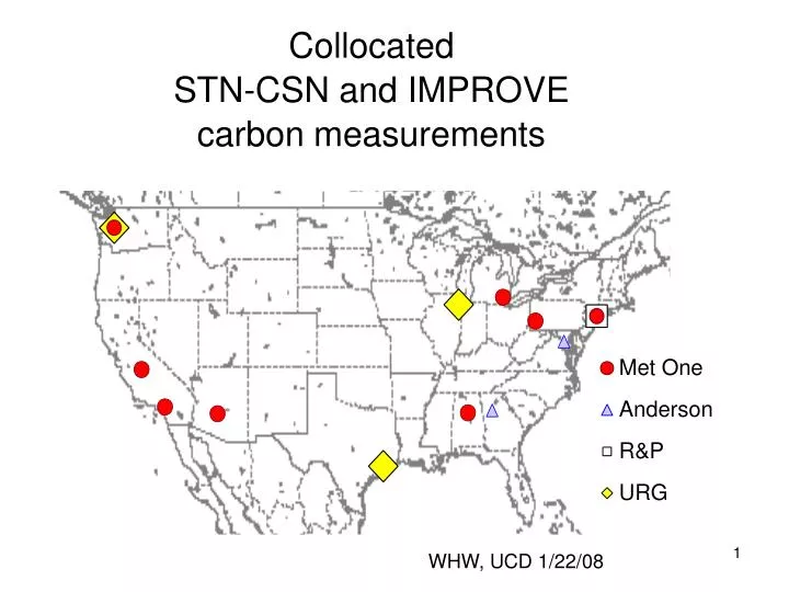
Collocated STN-CSN and IMPROVE carbon measurements WHW, UCD 1/22/08. IMPROVE analytical upgrade. EXPECTIONS & WORKING ASSUMPTIONS – analysis : Analytical methods agree for TC = OC + EC: TC CSN = TC IMP i.e. , carbon itself is measured unambiguously.

E N D
Collocated STN-CSN and IMPROVE carbon measurements WHW, UCD 1/22/08
EXPECTIONS & WORKING ASSUMPTIONS – analysis: Analytical methods agree for TC = OC + EC: TCCSN = TCIMP i.e., carbon itself is measured unambiguously. The relationship between the splits is linear and homogeneous: OC OCmeasured OCmeasured = (1-f)OC + gEC EC ECmeasured ECmeasured = fOC + (1-g)EC IMPROVE’s f and g may differ between old and new TOR analyses.
EXPECTATIONS & WORKING ASSUMPTIONS – sampling: The collected sample may be affected by filter artifacts (FA) and sampling artifacts (SA): C = (1-BSA)[C]V + AFA, BSA> 0 and AFA> 0 The filter and sampling artifacts for EC are negligible in both networks: EC = [EC]V (BSA = 0 and AFA = 0) These assumptions lead us to expect an ‘unadjusted’ value (reported by CSN) of: TC/V = OC/V + EC/V = (1-BSA)[OC] + AFA/V + [EC] = [TC] – BSA[OC] + AFA/V
Out-of-range points are always plotted at the appropriate boundary. EC Each point is the median from all observations on days -3, 0, +3 by the indicated sampler.
TC inverse of previous ratio Note the switch from IMPROVE / CSN to CSN / IMPROVE. (Both plots show the larger measurement on top.)
TC difference, not ratio Neither ratio nor difference is quite ‘right’ for a relationship of the form [CSN] = a + b[IMPROVE].
For EC, the systematic differences between CSN and IMPROVE, and between old and new IMPROVE, seem to be multiplicative.
For TC, the difference between CSN and IMPROVE appears to include an additive offset in addition to a multiplicative factor. There is no obvious difference between old and new IMPROVE.
2005-6 For EC, the difference between CSN and IMPROVE shows little dependence on the CSN sampler, suggesting that it is mainly analytical.
2005-6 For TC, the difference between CSN and IMPROVE clearly does vary with the CSN sampler.
2005-6 Site-specific differences between CSN and IMPROVE are evident only at Phoenix, where the MetOne - IMPROVE TC difference tends to be higher than it is elsewhere.
Phoenix, 2004-6 A collocated IMPROVE monitor has operated at Phoenix since March 2004. These plots compare the two collocations on days with observations from both. Nothing out of the ordinary is evident.
RECALL OUR WORKING ASSUMPTION: TC/V = [TC] – BSA[OC] + AFA/V (i) The MetOne face velocity (6.7 L/min through a 47 mm filter) is much lower than the IMPROVE face velocity (~22.8 L/min through a 25 mm filter). (ii) Reported IMPROVE concentrations are ‘corrected’ for the filter artifact. It will simplify our interpretation if we accordingly neglect (i) the MetOne sampling artifact and (ii) the IMPROVE filter artifact. Then [TC]IMP = [TC] – BIMP[OC] and [TC]CSN = [TC] + ACSN/VMetOne. Solving for [TC] in both expressions and equating the two solutions yields [TC]CSN = [TC]IMP + BIMP[OC] + ACSN/VMetOne Estimate OC: ~ [TC]IMP + BIMP*[OC]IMP + ACSN/VMetOne = [EC]IMP + (1+BIMP*)[OC]IMP + ACSN/VMetOne
EXPECTATION: [TC]CSN = [EC]IMP + (1+BIMP*)[OC]IMP + ACSN/VMetOne OLS REGRESSION: [TC]CSN = (1+bEC)[EC]IMP + (1+bOC)[OC]IMP + a1 +…+ a12 + e 2005-6 observations at 7 MetOne sites (excluding Phoenix): bEC = 0.008 (+/-0.05) no sampling artifact for IMPROVE EC bOC = 0.22 (+/-0.03) ~ 20% sampling loss for IMPROVE OC rms(e) = 0.9 ug/m3 (r2 = 0.986, n = 779) amm next slide
OLS REGRESSION FOR EC: [EC]CSN = (1-g)[EC]IMP + f[OC]IMP + a1 +…+ a12 + e 2005-6 observations at 7 MetOne sites (excluding Phoenix): g = 0.40 (+/-0.02) f = 0.03 (+/-0.01) rms(e) = 0.3 ug/m3 (r2 = 0.942, n = 779) amm: mixed signs, marginal significance
‘REVIEW OF EVIDENCE FOR DIFFERENCES’: • Observed differences • Changed at 2004 2005 TOR transition • Vary with CSN sampler • Suggest a seasonally varying additive artifact in CSN OC (relative to IMPROVE) • Suggest a multiplicative negative artifact in IMPROVE OC (relative to CSN)
The 779 MetOne observations from 2005-6 at seven sites can be linearly transformed into IMPROVE values with rms errors of EC: 0.4 ug/m3 (27% of mean value) TC: 0.8 ug/m3 (16% of mean value)