Download
1 / 30
300 likes | 343 Views
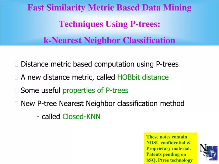
Fast Similarity Metric Based Data Mining Techniques Using P-trees: k-Nearest Neighbor Classification. Distance metric based computation using P-trees A new distance metric, called HOBbit distance Some useful properties of P-trees New P-tree Nearest Neighbor classification method

E N D
Fast Similarity Metric Based Data Mining Techniques Using P-trees: k-Nearest Neighbor Classification • Distance metric based computation using P-trees • A new distance metric, called HOBbit distance • Some useful properties of P-trees • New P-tree Nearest Neighbor classification method - called Closed-KNN These notes contain NDSU confidential & Proprietary material. Patents pending on bSQ, Ptree technology
Data Mining extracting knowledge from a large amount of data Useful Information (sometimes 1 bit: Y/N) More data volume = less information Data Mining Raw data Information Pyramid Functionalities: feature selection,association rule mining, classification & prediction, cluster analysis, outlier analysis
Classification Training data: Class labels are known and supervise the learning Feature1 Feature2 Feature3 Class a1 b1 c1 A a2 b2 c2 A a3 b3 c3 B Sample with unknown class: Classifier Predicted class Of the Sample a b c Predicting the class of a data object also called Supervised learning Eager classifier: Builds a classifier model in advance e.g. decision tree induction, neural network Lazy classifier: Uses the raw training data e.g. k-nearest neighbor
Clustering (unsupervised learning – cpt 8) A two dimensional space showing 3 clusters • The process of grouping objects into classes, • with the objective: the data objects are • similar to the objects in the same cluster • dissimilar to the objects in the other clusters. • Clustering is often calledunsupervised learning • or unsupervised classification • the class labels of the data objects are unknown
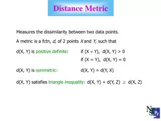
Distance Metric (used in both classification and clustering) Measures the dissimilarity between two data points. A metric is a fctn, d, of 2 n-dimensional points X and Y, such that d(X, Y)is positive definite: if (X Y), d(X, Y) > 0 if (X = Y), d(X, Y) = 0 d(X, Y) issymmetric: d(X, Y) = d(Y, X) d(X, Y) satisfies triangle inequality:d(X, Y) + d(Y, Z) d(X, Z)
Various Distance Metrics Minkowski distance or Lp distance, Manhattan distance, (P = 1) Euclidian distance, (P = 2) Max distance, (P = )
An Example Y (6,4) Z X (2,1) A two-dimensional space: Manhattan, d1(X,Y)= XZ+ ZY =4+3 = 7 Euclidian, d2(X,Y)= XY = 5 Max, d(X,Y)= Max(XZ, ZY) = XZ = 4 d1d2 d For any positive integer p,
Some Other Distances Canberra distance Squared cord distance Squared chi-squared distance
HOBbit Similarity Bit position: 1 2 3 4 5 6 7 8 1 2 3 4 5 6 7 8 x1: 0 1 10 1 0 0 1 x2: 0 1 0 11 1 0 1 y1: 0 1 11 1 1 0 1 y2: 0 1 0 1 0 0 0 0 HOBbitS(x1, y1) = 3 HOBbitS(x2, y2) = 4 Higher Order Bit (HOBbit) similarity: HOBbitS(A, B) = A, B: two scalars (integer) ai, bi :ith bit of A and B (left to right) m : number of bits
HOBbit Distance (related to Hamming distance) The previous example: Bit position: 1 2 3 4 5 6 7 8 1 2 3 4 5 6 7 8 x1: 0 1 10 1 0 0 1 x2: 0 1 0 11 1 0 1 y1: 0 1 11 1 1 0 1 y2: 0 1 0 1 0 0 0 0 HOBbitS(x1, y1) = 3 HOBbitS(x2, y2) = 4 dv(x1, y1) = 8 – 3 = 5 dv(x2, y2) = 8 – 4 = 4 The HOBbit distance between two pointsX and Y: In our example (considering 2-dimensional data): dh(X, Y) = max (5, 4) = 5 The HOBbit distance between two scalar value A and B: dv(A, B)= m – HOBbit(A, B)
HOBbit Distance Is a Metric HOBbit distance is positive definite if (X = Y), = 0 if (XY), > 0 HOBbit distance is symmetric HOBbit distance holds triangle inequality
Neighborhood of a Point 2r 2r 2r 2r X X X X T T T T Neighborhood of a target point, T, is a set of points, S, such thatXSif and only if d(T, X) r Manhattan Euclidian Max HOBbit If Xis a point on the boundary, d(T, X) = r
Decision Boundary Manhattan Euclidian Max Max Euclidian Manhattan > 45 < 45 X A A A A A R1 B B B B B d(A,X) d(B,X) R2 D decision boundary between points A and B, is the locus of the point X satisfying d(A, X) = d(B, X) Decision boundary for HOBbit Distance is perpendicular to axis that makes max distance Decision boundaries for Manhattan, Euclidean and max distance
Minkowski Metrics Lp-metrics (aka: Minkowski metrics) dp(X,Y) = (i=1 to n wi|xi - yi|p)1/p (weights, wi assumed =1)Unit DisksDividing Lines p=1 (Manhattan) p=2 (Euclidean) p=3,4,… . . Pmax (chessboard) P=½,⅓, ¼, … dmax≡ max|xi - yi| d≡ limp dp(X,Y). Proof (sort of) limp { i=1 to n aip }1/p max(ai) ≡b. For p large enough, other aip << bp since y=xp increasingly concave, so i=1 to n aip k*bp(k=duplicity of b in the sum), so {i=1 to n aip }1/p k1/p*b and k1/p1
P>1 Minkowski Metrics q x1 y1 x2 y2 e^(LN(B2-C2)*A2)e^(LN(D2-E2)*A2) e^(LN(G2+F2)/A2) 2 0.5 0 0.5 0 0.25 0.25 0.7071067812 4 0.5 0 0.5 0 0.0625 0.0625 0.5946035575 9 0.5 0 0.5 0 0.001953125 0.001953125 0.5400298694 100 0.5 0 0.5 0 7.888609E-31 7.888609E-31 0.503477775 MAX 0.5 0 0.5 0 0.5 2 0.70 0 0.7071 0 0.5 0.5 1 3 0.70 0 0.7071 0 0.3535533906 0.3535533906 0.8908987181 7 0.70 0 0.7071 0 0.0883883476 0.0883883476 0.7807091822 100 0.70 0 0.7071 0 8.881784E-16 8.881784E-16 0.7120250978 MAX 0.70 0 0.7071 0 0.7071067812 2 0.99 0 0.99 0 0.9801 0.9801 1.4000714267 8 0.99 0 0.99 0 0.9227446944 0.9227446944 1.0796026553 100 0.99 0 0.99 0 0.3660323413 0.3660323413 0.9968859946 1000 0.99 0 0.99 0 0.0000431712 0.0000431712 0.9906864536 MAX 0.99 0 0.99 0 0.99 2 1 0 1 0 1 1 1.4142135624 9 1 0 1 0 1 1 1.0800597389 100 1 0 1 0 1 1 1.0069555501 1000 1 0 1 0 1 1 1.0006933875 MAX 1 0 1 0 1 2 0.9 0 0.1 0 0.81 0.01 0.9055385138 9 0.9 0 0.1 0 0.387420489 0.000000001 0.9000000003 100 0.9 0 0.1 0 0.0000265614 ************** 0.9 1000 0.9 0 0.1 0 1.747871E-46 0 0.9 MAX 0.9 0 0.1 0 0.9 2 3 0 3 0 9 9 4.2426406871 3 3 0 3 0 27 27 3.7797631497 8 3 0 3 0 6561 6561 3.271523198 100 3 0 3 0 5.153775E+47 5.153775E+47 3.0208666502 MAX 3 0 3 0 3 6 90 0 45 0 531441000000 8303765625 90.232863532 9 90 0 45 0 3.874205E+17 7.566806E+14 90.019514317 100 90 0 45 0 **************************** 90 MAX 90 0 45 0 90
P<1 Minkowski Metrics d 1/p(X,Y) = (i=1 to n |xi - yi|1/p)p P<1 p=0 (lim as p0) doesn’t exist (Does not converge.) q x1 y1 x2 y2 e^(LN(B2-C2)*A2) e^(LN(D2-E2)*A2) e^(LN(G2+F2)/A2) 1 0.1 0 0.1 0 0.1 0.1 0.2 0.8 0.1 0 0.1 0 0.1584893192 0.1584893192 0.237841423 0.4 0.1 0 0.1 0 0.3981071706 0.3981071706 0.5656854249 0.2 0.1 0 0.1 0 0.6309573445 0.6309573445 3.2 0.1 0.1 0 0.1 0 0.7943282347 0.7943282347 102.4 .04 0.1 0 0.1 0 0.9120108394 0.9120108394 3355443.2 .02 0.1 0 0.1 0 0.954992586 0.954992586 112589990684263 .01 0.1 0 0.1 0 0.977237221 0.977237221 1.2676506002E+29 2 0.1 0 0.1 0 0.01 0.01 0.1414213562 q x1 y1 x2 y2 e^(LN(B2-C2)*A2) e^(LN(D2-E2)*A2) e^(LN(G2+F2)/A2) 1 0.5 0 0.5 0 0.5 0.5 1 0.8 0.5 0 0.5 0 0.5743491775 0.5743491775 1.189207115 0.4 0.5 0 0.5 0 0.7578582833 0.7578582833 2.8284271247 0.2 0.5 0 0.5 0 0.8705505633 0.8705505633 16 0.1 0.5 0 0.5 0 0.9330329915 0.9330329915 512 0.04 0.5 0 0.5 0 0.9726549474 0.9726549474 16777216 0.02 0.5 0 0.5 0 0.9862327045 0.9862327045 5.6294995342E+14 0.01 0.5 0 0.5 0 0.9930924954 0.9930924954 6.3382530011E+29 2 0.5 0 0.5 0 0.25 0.25 0.7071067812 q x1 y1 x2 y2 e^(LN(B2-C2)*A2) e^(LN(D2-E2)*A2) e^(LN(G2+F2)/A2) 1 0.9 0 0.1 0 0.9 0.1 1 0.8 0.9 0 0.1 0 0.9191661188 0.1584893192 1.097993846 0.4 0.9 0 0.1 0 0.9587315155 0.3981071706 2.14447281 0.2 0.9 0 0.1 0 0.9791483624 0.6309573445 10.8211133585 0.1 0.9 0 0.1 0 0.9895192582 0.7943282347 326.27006047 0.04 0.9 0 0.1 0 0.9957944476 0.9120108394 10312196.9619 0.02 0.9 0 0.1 0 0.9978950083 0.954992586 341871052443154 0.01 0.9 0 0.1 0 0.9989469497 0.977237221 3.8259705676E+29 2 0.9 0 0.1 0 0.81 0.01 0.9055385138
Min dissimilarity function The dmin function (dmin(X,Y) = min i=1 to n|xi - yi| is strange. It is not a psuedo-metric. The Unit Disk is: And the neighborhood of the blue point relative to the red point (dividing nbrhd - those points closer to the blue than the red). Major bifurcations! http://www.cs.ndsu.nodak.edu/~serazi/research/Distance.html
Other Interesting Metrics Canberra metric: dc(X,Y) = (i=1 to n |xi – yi| / (xi + yi) - normalized manhattan distance Square Cord metric: dsc(X,Y) = i=1 to n( xi – yi )2 - Already discussed as Lp with p=1/2 Squared Chi-squared metric: dchi(X,Y) = i=1 to n (xi – yi)2/ (xi + yi) HOBbit metric (Hi Order Binary bit) dH(X,Y) = max i=1 to n{n – HOB(xi - yi)} where, for m-bit integers, A=a1..am and B=b1..bm HOB(A,B) = max i=1 to m {s: i(1 i s ai=bi)} (related to Hamming distance in coding theory) Scalar Product metric: dchi(X,Y) = X • Y = i=1 to n xi * yi Hyperbolic metrics: (which map infinite space 1-1 onto a sphere) Which are rotationally invariant? Translationally invariant? Other?
Notations rc(P) : root count of P-tree, P N :number of pixels n : number of bands m :number of bits P1& P2:P1AND P2 (alsoP1^ P2) P1 | P2 :P1OR P2 P´:COMPLEMENT P-tree of P Pi, j : basic P-tree for band-i bit-j. Pi(v) : value P-tree for value v of band i. Pi([v1, v2]) : interval P-tree for interval [v1, v2] of band i. P0 : is pure0-tree, a P-tree having the root node which is pure0. P1 : is pure1-tree, a P-tree having the root node which is pure1.
Properties of P-trees 1. a) b) 2. a) b) c) d) 3. a) b) c) d) • 4. rc(P1 | P2)= 0 iff rc(P1)= 0andrc(P2) = 0 • v1 v2 rc{Pi(v1)& Pi(v2)} = 0 • rc(P1 | P2) = rc(P1) + rc(P2) - rc(P1 & P2) • rc{Pi (v1) | Pi(v2)} = rc{Pi(v1)} + rc{Pi(v2)}, where v1 v2
k-Nearest Neighbor Classification and Closed-KNN T 1) Select a suitable value for k 2) Determine a suitable distance metric 3) Find k nearest neighbors of the sample using the selected metric 4) Find the plurality class of the nearest neighbors by voting on the class labels of the NNs 5) Assign the plurality class to the sample to be classified. T is the target pixels. With k = 3, to find the third nearest neighbor, KNN arbitrarily select one point from the bdry line of the nhbd Closed-KNN includes all points on the boundary Closed-KNN yields higher classification accuracy than traditional KNN
SearchingNearestNeighbors We begin searching by finding the exact matches. Let the target sample, T = <v1, v2, v3, …, vn> The initial neighborhood is the point T. We expand the neighborhood along each dimension: along dim-i, [vi] expanded to the interval [vi – ai , vi+bi], for some pos integers ai and bi. Continue expansion until there are at least k points in the neighborhood.
HOBbit Similarity Method for KNN In this method, we match bits of the target to the training data First, find those matching in all 8 bits of each band (exact matches) let, bi,j = jth bit of the ith band of the target pixel. Define target-Ptree, Pt:Pti,j = Pi,j , if bi,j = 1 = Pi,j , otherwise And precision-value-Ptree, Pvi,1j = Pti,1 & Pti,2 & Pti,3 & … & Pti,j
An Analysis of HOBbit Method • Let ith band value of the target T, vi= 105 = 01101001b • [01101001] [105, 105] • 1st expansion • [0110100-] = [01101000, 01101001] = [104, 105] • 2nd expansion • [011010--] = [01101000, 01101011] = [104, 107] • Does not expand evenly in both side: • Target = 105 and center of [104, 111] = (104+107) / 2 = 105.5 • And expands by power of 2. • Computationally very cheap
Perfect Centering Method Max distance metric provides better neighborhood by - keeping the target in the center - and expanding by 1 in both side Initial neighborhood P-tree (exact matching): Pnn = P1(v1)& P2(v2)& P3(v3) & … &Pn(vn) If rc(Pnn) < k , Pnn = P1(v1-1, v1+1)& P2(v2-1, v2+1)& … & Pn(vn-1, vn+1) If rc(Pnn) < k , Pnn = P1(v1-2, v1+2)& P2(v2-2, v2+2)& … & Pn(vn-2, vn+2) Computationally costlier than HOBbit Similarity method But a little better classification accuracy Let, Pc(i) is the value P-trees for the class i Plurality class =
Performance Experimented on two sets of Arial photographs of The Best Management Plot (BMP) of Oakes Irrigation Test Area (OITA), ND Data contains 6 bands: Red, Green, Blue reflectance values, Soil Moisture, Nitrate, and Yield (class label). Band values ranges from 0 to 255 (8 bits) Considering 8 classes or levels of yield values: 0 to 7
Performance – Accuracy 1997 Dataset:
Performance - Accuracy (cont.) 1998 Dataset:
Performance - Time 1997 Dataset: both axis in logarithmic scale
Performance - Time (cont.) 1998 Dataset : both axis in logarithmic scale