Download
1 / 42
420 likes | 513 Views
3). Dielectric phenomena. Microscopic picture – change in charge density when field is applied. r ( r ) Electronic charge density. No E field E field on. E. Dr ( r ) Change in electronic charge density Note dipolar character. r. - +. Dipole Moments of Atoms.

E N D
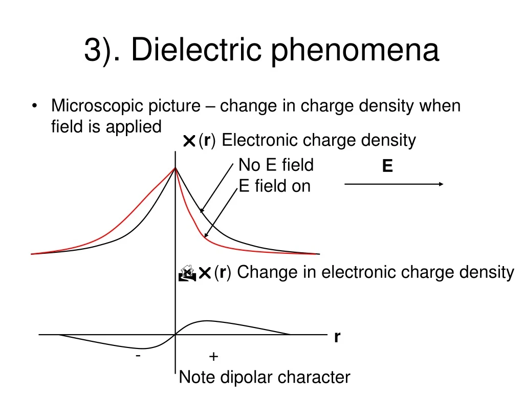
3). Dielectric phenomena • Microscopic picture – change in charge density when field is applied r(r) Electronic charge density No E field E field on E Dr(r) Change in electronic charge density Note dipolar character r - +
Dipole Moments of Atoms • Total electronic charge per atom Z = atomic number • Total nuclear charge per atom • Centre of mass of electric or nuclear charge distribution • Dipole moment Zea
z r+ r- r q+ a/2 x a/2 p q- Electrostatic potential of point dipole • +/- charges, equal magnitude, q, separation a • axially symmetric potential (z axis)
Equipotential lines: dipole • Contours on which electric potential is constant Equipotential lines perp. to field lines
Field lines: point dipole • Generated from r k f q q j f i ← NB not a point dipole
No E field E field on Insulators vs metals • Insulator • Localised wave functions • Metal • Delocalised wave functions
E E E E p P P + - Polarisation • Polarisation P = dipole moment p per unit volume Cm/m3 = Cm-2 • Mesoscopic averaging: P is a constant vector field for a uniformlypolarised medium • Macroscopic chargessp in a uniformly polarised medium sp = ___? dS
EDep + - E E Depolarising electric field • Depolarising electric field EDep in uniformly polarised ∞ slab • Macroscopic electric field EMac= E + EDep EDep = sP/2o +sP/2o EDep= -P/o EMac = E - P/o EMac + -
Relative Permittivity and Susceptibility • EMac = E– P/ o = (splates – P)/ o in magnitude • oE = oEMac + PP = ocEEMac • oE = oEMac + ocEEMac = o (1 + cE)EMac = oEMac • EMac = E/ • E = eEMac • Dielectric constant (relative permittivity) = 1 + cE • Typical values: silicon 11.8, diamond 5.6, vacuum 1 • Dielectric susceptibilty cE
_ _ _ _ + + + + E Polar dielectrics • molecules possess permanent dipole moment • in the absence of electric field, dipoles randomly oriented by thermal motion • hence, no polarisation. e.g. HCl and H2O …..but not CS2 no net dipole moment zero field, random preferential alignment net P=0 but P Np
+ + Edip Eappl Eappl _ _ Effect of orientation on net field • Effect of alignment is to reduce the net field • Tendency to align is opposed by thermal effects • Balance is determined by Boltzmann statistics • Key factor is ratio of the potential energy of the dipole (U) to the temperature (T), which enters as exp(-U/kT)
+ E _ q Potential energy of dipole in E field • Potential energy U (U c.f.W from before) when charge density of molecule (r) is in slowly spatially varying external potential (No factor of ½ c.f. W) If q = 0, leading term is –p.E = -pEcosq
Number Distribution function Angular distribution function: N(q) (no E field), N’(q) (E field) Number of dipoles oriented betweenqandq+dq: N(q)dq Total number of dipoles N E||z no E field dW q f E field on
Number Distribution function • Total number of dipoles N
E 1/T Susceptibility of polar dielectric • Molecules acquire induced dipole moment through: - reorientation - polarisation of molecular charge (polar or nonpolar molecules)
P Np pE/kT The Langevin Equation When U/kT is not small, integration of N(q)dq yields: Plotting P vs pE/kT shows two distinct regimes: • High E, low T: all dipoles aligned: • Low E, high T: small U/kT approximation:
dS + - dq q - - + + q R - + p - q P, E cos(p - q)= - cos q Clausius-Mossotti equation • Relationship betweenerand polarisability densityNa including local fields • Neglected local field for polar dielectrics (dilute gases) • Each molecule, atom, etc. located in spherical cavity • C-M local field is external field + field due to polarisation charges on cavity surfaceEloc = E + Epol • pol = P.dS P dS P.dS= - P dS cosq ring area element = 2pRsinq Rdq
Clausius-Mossotti equation • Charge on ring area element - P dS cosq = -eo cEE 2pRsinq Rdq cosq • Contribution to field at centre of cavity from pol on ring eo cEE 2pRsinq Rdq cosq/(4peo R2) = cEE sinq cosq dq/2 • Field || P due to all charge on cavity surface Epol= cEE/3 • Local field Eloc = E + Epol= (1+ cE/3)E • P = eoNaEloc = eoNa(1+ cE/3)E (in cavity) • P = eo cEE (in bulk) • Na(1+ cE/3)= cE • Na= cE / (1+ cE/3)Na/3 = (er – 1)/(er + 2) since er = 1 + cE
E P P + - Non-uniform polarisation • Uniform polarisation surface charges only • Non-uniform L polarisation bulk charges also Displacements of positive charges Accumulated charges + - + -
(x,y,z) (x+Dx,y,z) Non-uniform polarisation Box with origin of local axes at (x,y,z), volume DxDyDz Charge crossing area dS = P.dS Charge entering LH yz face Charge exiting RH yz face Net charge entering box Total charge including zx and xy pairs of faces
Added (free) charge Polarisation (bound) charge response of dielectric to added charge Electric displacement D • What happens when a charge is added to a neutral dielectric ? • Two types of charge: • Those due to polarisation (bound charges) • Those due to extra charges (free charges) (charge injection by electrode, etc) • Total charge
Electric displacement D • Gauss’s Law • Displacement: a vector whose div equals free charge density • Units: C·m-2 (same as P) • D relates E and P • D = eoE + P is a constitutive relation • Can solve for D field and implicitly include E and P fields
Validity of expressions • Always valid: Gauss’ Law for E, P and D relation D =eoE + P • Limited validity: Expressions involving er and E • Have assumed that Eis a simple number: P = eo EE only true in LIH media: • Linear: Eindependent of magnitude of E interesting media “non-linear”: P = EeoE + 2EeoEE + …. • Isotropic: Eindependent of direction of E interesting media “anisotropic”: Eis a tensor (generates vector) • Homogeneous: uniform medium (spatially varying er)
+ - E Emac=E/er E + - D = eoE D = eoE + P =eoerEmac D = eoE Boundary conditions on D and E • Simplest example – charged capacitor with dielectric • D is continuous ┴ boundaries (no free charges there) • E is discontinuous ┴ boundaries
1 2 (E1,D1) q1 (E2,D2) S q2 Boundary conditions on D • We know that • Absence of free charges at boundary D1 cosq1 S – D2 cosq2 S = 0 D1 cosq1 = D2 cosq2 D1┴ = D2 ┴ Perpendicular component of D is continuous • Presence of free charges at boundary D1 cosq1 S – D2 cosq2 S = S sf D1┴ = D2 ┴ + sf Discontinuity in perpendicular component of D is free charge areal density
q1 dℓ1 (E1,D1) 1 B A C 2 q2 (E2,D2) dℓ2 Boundary Conditions on E • We know that for an electrostatic E field • E and D are constant along the horizontal sides of C in regions 1 or 2 • Sides of C thin enough to make no contribution • Parallel component of E is continuous across boundary
q1 1 2 q2 Interface between 2 LIH media LIH D = ereoE E and D bend at interface
Energy of free charges in dielectric In vacuum Assembling free charges in a dielectric
Method of Images Derives from Uniqueness Theorem: “only one potential Satisfies Poisson’s Equation and given boundary conditions” Can replace parts of system with simpler “image” charge arrangements, as long as same boundary conditions satisfied Method exploits: • Symmetry • Gauss’s Law Image charges reproduce BC f or f specified
+Q +Q -Q Basic Image Charge Example Consider a point charge near an infinite, grounded, conducting plate: induced -ve charge on plate; potential zero at plate surface Complex field pattern, combining radial (point charge +Q) and planar (conducting plate) symmetries, can also be viewed as half of pattern of 2 point charges (+Q and -Q) of equal magnitude and opposite sign!
Basic Image Charge continued Arrangement is equivalent because it keeps the same boundary condition (potential zero on plate and zero potential on the median line). Point charge -Q is located same distance behind, like an image in a plane mirror. The resulting field is easy to calculate (vector sum of fields of 2 point charges of equal and opposite sign) Field lines must be normal to surface of conductor Also easy to calculate the induced -ve charge on plate!
E+ E E- r q +Q -Q D Distribution of induced charge Induced charge is related to the outwardE field at the surface: Find E using image charge (-ve and varying with r)
ds s r s D Total induced charge Introduce parameter s sind has azimuthal symmetry: consider elemental annulus, radius s, thickness ds
Total induced charge: implications 2 conclusions from the result: • Induced charge equals the negative of original point charge - trivially true in this case only! • Induced charge equals the image charge - generally true! Consider Gauss’s Law, concept of enclosed charge Must not try to determine E in the region of image charge! In this case (behind infinite conductor) it is zero, which is not the answer the image charge would yield
- a +Q - - - D Point charge near grounded conducting sphere By comparison with previous example: • Distance D to centre of symmetry, radius a • Image (charge) location • -ve induced charge predominantly on side facing +Q • Boundary condition, zero potential on sphere surface Expect image charge will be a point charge on centre line, left of centre of sphere, magnitude not equal to Q, call it Q
Q Q P2 P1 b D Point charge near grounded conducting sphere Q distance b from centre, =0at symmetry points P1 and P2
Q Q Q V Point charge near floating conducting sphere On its own, floating the sphere at V relative to ground results in uniform +ve charge density over the surface. In the presence of Q, induced -ve charge predominantly on left; this complex system easily solved by 2 image charges:
Q Q Q Point charge near isolated conducting sphere With no connection to ground, the sphere is at an unknown non-zero potential ; easily solved by same 2 image charges: the potential is still determined by Q but in this case, the sphere is overall neutral: Q+Q=0 (same potential as if sphere was absent!)
Q e =1 r q D Eno s sb,ind Eni e = er Point charge near LIH dielectric block • Q polarises dielectric and produces bound surface charge sb,ind • sb,ind = P.n = eo(er-1)Eni Eni normal component of E inside • sb,ind negative if Q positive
E+ E r E- r q +Q Point charge near LIH dielectric block • Image charge for Eno • Image charge for Eni E+ E r r q
Point charge near LIH dielectric block (see Lorrain,Corson & Lorrain pp 212-217) Outside: remove dielectric block and locate image charge Q a distance D behind Inside: remove dielectric block and replace original point charge Q by Q
Point charge near LIH dielectric block contrasting E field patterns conductor dielectric note dielectric distorted outside but radial inside