Download
1 / 23
240 likes | 394 Views
Computer simulation. Sep. 9 , 2013. QUIZ. Determine whether the following experiments have discrete or continuous out comes. A fair die is tossed and the number of dots on the face noted. Identify the random experiment, the set of outcomes, and the probabilities of each possible outcome.

E N D
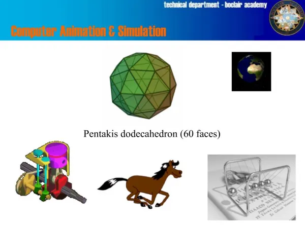
Computer simulation Sep. 9, 2013
QUIZ • Determine whether the following experiments have discrete or continuous out comes • A fair die is tossed and the number of dots on the face noted. Identify the random experiment, the set of outcomes, and the probabilities of each possible outcome.
Introduction • Introduce computer simulations (ComSim) • Show how to use ComSim to • provide counter examples (can’t be used to prove theorems) • simulate the outcomes of a discrete random variable • Give examples of typical ComSim used in probability • Monte Carlo computer approaches are a broad class of computationa algorithms that rely on repeated random sampling to obtain numerical results; i.e., by running simulations many times over in order to calculate those same probabilities heuristically just like actually playing and recording your results in a real casino situation: hence the name.
Why Use Computer Simulations? • To provide counterexamples to proposed theorems • To build intuition by experimenting with random numbers • To lend evidence to a conjecture (an unproven proposition).
Building intuition using ComSim • If U1and U2 are the outcomes of two experiments each is a number from 0 to 1. • What are the probabilities of X = U1 + U2? The mathematical answer will be given in later lectures • Assume X is equally likely to be in the interval [0,2]. • Let’s check if our intuition is correct by carrying out a ComSim. • Generate values U1and U2 them sum them up to obtain X. • Repeat this procedure M times. • Build a histogram which gives the number of outcomes in each bin.
Building intuition using ComSim • Assume the following M = 8 outcomes were obtained {1.7, 0.7, 1.2, 1.3, 1.8, 1.4, 0.6, 0.4} • Choosing the four bins [0, 0.5], (0.5, 1], (1, 1.5], (1.5, 2] we get
Building intuition using ComSim M = 1000 • It is clear that values of X are not equally likely. More probable
Building intuition using ComSim • The probabilities are higher near one because there are more ways to obtain these values. • X = 2 can be obtained from U1 = U2 = 1, but X = 1 can be obtained from U1 = U2 = ½ or U1 = ¼, U2 = ¾, or U1 = ¾, U2 = ¼, etc.
Building intuition using ComSim • The result can be extended to the addition of three of more experimental outcomes. • Define X3 = U1 + U2 + U3and X4 = U1 + U2 + U3+ U4. • The histogram appears more like a bell-shaped(Gaussian) curve • Conjecture: as we add more outcomes we obtain Gaussian
ComSim of Random Phenomena • A random variable (RV) Xis a variable whose value is subject to variations due to chance. • Discrete : the number of dots on a die X can take on the values in the set {1, 2, 3, 4, 5, 6} • Continuous : the distance of a dart from the center of the dartboard radius r = 1. {r : 0 ≤ r ≤ 1} • To determine various properties of X we perform a number of experiments (trials) that is denoted by M. • Assume that X = {x1, x2, …,xN} with probabilities {p1, p2, …,pN}.
ComSim of Random Phenomena • As an example if N = 3 we can generate M values of X by using the following code segment. • For a continuous RVX that is Gaussian we can use the code
Determining Characteristics of RV • The probability of the outcomes in the discrete case and the PDF in the continuous case are complete description of a random phenomenon. • Consider a discrete RV, the outcome of a coin toss. • Let X be 0 if a tail is observed with probability p and let X be 1 if head is observed with probability 1 – p. p is slightly large than the true value of 0.4 due to imperfection of the random number generator • To determine the probability of head we could toss a coin a large number of times and estimate p. We can simulate this result by using ComSim and estimate p. However, it is not always correct.
Probability density function(PDF) estimation • PDF can be estimated by first finding the histogram and then dividing the number of outcomes in each bin by Mto obtain the probability. • The to obtain the PDF pX(x) recall that the probability of X taking on a value in an interval is found as the area under the PDF • and if a = x0 – Δx/2 and b= x0 – Δx/2 ,where Δxis small, then • Hence, we need only divide the estimated probability by the bin width Δx.
Probability density function(PDF) estimation • Applying this estimation procedure to the set of simulated outcomes that has Gaussian PDF we are able to obtain estimated PDF.
Probability of an interval • To determine P[a ≤ X ≤ b] we need to generate M realizations of X, then count the number of outcomes that fall into the [a, b] interval and divide by M. • If we let a = 2, and b = ∞, then we should obtain the value (using numerical integration) • And therefore very few realizations can be expected to fall in this interval.
Determining Characteristics of RV • Average(mean) value • A mean value of transformed variable f(x) = x2
Multiple random variables • Consider an experiment the choice of a point in the square {(x, y) : 0 ≤ x ≤ 1, 0 ≤ y ≤ 1} according to some procedure. So it yields two RVs or the vector [X1, X2]T. • This procedure may or may not cause the value of x1 to depend on the value of x2. No dependency Dependency • There is a strong dependency, because if for example x1 = 0.5, then x2 would have to lie in the interval [0.25, 0.75].
Multiple Random Variables • Consider the two random vectors, where Ui is generated using rand. • Then the result of M = 1000 realizations are the scatter diagrams No dependency Dependency
Monte Carlo simulation • Consider a circle inscribed in a unit square. Given that the circle and the square have a ratio of areas that is π/4, the value of π can be approximated using a Monte Carlo method: • Draw a square on the ground, then inscribe a circle within it. • Uniformly scatter some objects of uniform size (grains of rice or sand) over the square. • Count the number of objects inside the circle and the total number of objects. • The ratio of the two counts is an estimate of the ratio of the two areas, which is π/4. Multiply the result by 4 to estimate π.
Digital Communications • In a phase-shift keyed (PSK) digital system a bit is communicated to receiver by sending • 0 : s0(t) = Acos(2πF0t + π) • 1 : s1(t) = Acos(2πF0t) • The receiver
Digital Communications • The input to the receiver is the noise corrupted signal where w(t) is the channel noise. • The output of the multiplier will be (ignoring the noise) Recall
Digital Communications • After the lowpass filter, which filters out the Acos(2πF0t) part of the signal and sampler we have • To model the channel noise we assume that the actual value ξ of observed is , where W is a Gaussian RV
Digital Communications • It is of interest to determine how the error depends on the signal amplitude A. • If A is a large positive amplitude, the chance that the noise will cause an error or equivalently, ξ ≤ 0,should be small. • The probability of error Pe = P[A/2 + W≤ 0] • Usually Pe = 10-7.