Download
1 / 57
590 likes | 900 Views
Computer Networking Packet Switching Networks. Dr Sandra I. Woolley. Contents. Packet switching and the network layer Structure of a packet switch Routing in packet networks Shortest path routing Distance Vector (Bellman-Ford) Link-State (Dijkstra). Packet Switching. t 1. t 0. Network.

E N D
Computer NetworkingPacket Switching Networks Dr Sandra I. Woolley
Contents • Packet switching and the network layer • Structure of a packet switch • Routing in packet networks • Shortest path routing • Distance Vector (Bellman-Ford) • Link-State (Dijkstra)
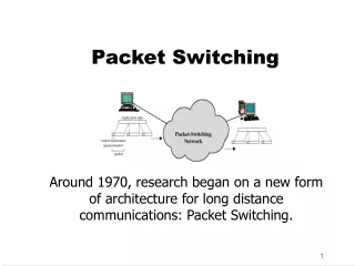
Packet Switching t1 t0 Network • Transfer of information as payload in data packets. • Packets undergo random delays and possible loss. • Different applications impose differing requirements on the transfer of information. • How do we get packets from here to there?
Network Layer • The network layer is the most complex layer. • Addressing needs to accommodate extremely large-scale networks and must work together with appropriate routing algorithms. • These two challenges, addressing and routing, are the essence of the network layer. • Addressing: where should information be directed to? • Routing: what path should be used to get information there?
Network Service Messages Messages Segments Transport layer Transport layer Network service Network service Network layer Network layer Network layer Network layer Data link layer Data link layer Data link layer Data link layer End system β End system α Physical layer Physical layer Physical layer Physical layer • The network layer can offers services to transport layer. • The network service can be connection-oriented or connectionless. Best-effort or delay/loss guarantees.
Complexity at the Edge or in the Core? • Complexity is best at the edge of the network. • Higher-level components at the ends are better positioned to check functionality and take corrective action. • Keeping the core of the network simple and adding the necessary complexity at the edges enhances scalability.
Network Layer Functions Essential • Routing: mechanisms for determining the set of best paths for routing packets requires the collaboration of network elements. • Forwarding: transfer of packets from NE (network element) inputs to outputs. • Priority and Scheduling: determining order of packet transmission in each NE. Optional • Congestion control, segmentation & reassembly, security.
Key Role of Routing • How to get packet from here to there? • The decentralized nature of the Internet makes routing a major challenge. • Interior gateway protocols (IGPs) are used to determine routes within a domain. • Exterior gateway protocols (EGPs) are used to determine routes across domains. • Routes must be consistent and produce stable flows. • Scalability required to accommodate growth. • The hierarchical structure of IP addresses is essential to keeping size of routing tables manageable.
The network service provided can be connection-oriented or connectionless. Connection-oriented - setting up a connection across the network before information can be transferred. Connectionless - does not involve setting up connections. Packets are routed independently until they reach their destination. Both approaches need packet switches to direct packets. Packet switches store and forward packets. Packet Switching Network User Transmission line Network Packet switch
Packet 1 Packet 1 Packet 2 Packet 2 Packet 2 Connectionless/Datagram Packet Switching • Source and destination addresses are in packet headers. • Connectionless (datagram) packets are routed independently. • Packets may arrive out of order.
Route is determined by table lookup. Routing decision involves finding next hop along the route to given destination. Routing table has an entry for each destination specifying the output port that leads to the next hop. Table size becomes problematic for very large numbers of destinations. Routing Tables in Datagram Networks Destination Output address port 0785 7 1345 12 1566 6 2458 12
Example: Internet Routing • Internet protocol uses datagram packet switching across networks • Networks are treated as data links • Hosts have two-part IP address: • Network address + Host address • Routers do table lookup on network address • This reduces size of routing table • In addition, network addresses are assigned so that they can also be aggregated • Discussed as CIDR in TCP/IP lectures
Virtual Circuit Packet Switching Packet Packet Packet Packet Virtual circuit • Virtual-circuit packet switching involves establishing a fixed path between source and destination. This is established prior to packet flow. • Routing tables are configured in every switch along the path. • All packets for a connection follow the same path. Packets arrive in sequence. • An abbreviated header identifies connection on each link. • Packets queue for transmission. • Variable bit rates possible, negotiated during call set-up.
Each input port of packet switch has a forwarding table. Lookup entry for VCI (virtual circuit identifier) of incoming packet. Determine output port (next hop) and insert VCI for next link. Very high speeds are possible. Table can also include priority or other information about how the packet should be treated. Virtual Circuit Forwarding Tables Input VCI Output port Output VCI 12 44 13 15 15 23 16 27 13 58 7 34
Packet Switch: Where Traffic Flows Meet • • • • • • • • • • Inputs contain multiplexed flows from access multiplexers and other packet switches. • Flows are demultiplexed at the input and forwarded to the correct output port. • Packets are buffered, prioritized, and multiplexed to output lines. 1 1 2 2 N N
“Unfolded*” View of Switch Ingress (receive) Line Cards Header processing Demultiplexing Routing in large switches Controller Routing in small switches Signalling and resource allocation (in connection-oriented mode) Internal configuration and maintenance Interconnection Fabric Transfer packets between line cards Egress (transmit) Line Cards Scheduling & priority Multiplexing *Each line card contains both inputs and outputs. Generic Packet Switch Controller 1 Line card 1 Line card 2 2 Line card Line card 3 3 Line card Interconnection fabric Line card … … … … N N Line card Line card Input ports Output ports Data path Control path (a)
Crossbar Switches (b) Output buffering (a) Input buffering • The crossbar is a higher-speed alternative to serially transferred interconnection fabrics which can cause bottlenecks. • Large switches built from crossbar and multistage space switches • Can buffer at input, output, or both (performance vs. complexity) Inputs Inputs 3 1 1 2 8 3 2 3 3 … … N N … … 1 2 3 N 1 2 3 N Outputs Outputs
Self-Routing Switches: A Banyan Switch Inputs Outputs 0 0 1 1 2 2 3 3 4 4 5 5 6 6 7 7 Stage 1 Stage 2 Stage 3 • Self-routing switches do not require a controller. • The output port number determines the route. • 101 → (1) lower port, (2) upper port, (3) lower port • In the example … 0=up and 1=down A banyan is a fig that grows on a host tree. Its roots twist down toward the ground. http://forest.puducherry.gov.in/forest/banyan%20tree.jpg
Routing in Packet Networks 1 3 6 4 2 Node (switch or router) 5 • There are three possible (loopfree) routes from 1 to 6: • 1-3-6, 1-4-5-6, 1-2-5-6 • But which is “best”? • Min delay? Min hop? Max bandwidth? Min cost? Max reliability?
Creating the Routing Tables • Need information on state of links. • Link up/down; congested; delay or other metrics • Need to distribute link state information using a routing protocol. • What information is exchanged? How often? • Exchange with neighbours; Broadcast or flood • Need to compute routes based on information. • Single metric; multiple metrics • Single route; alternate routes
Routing Algorithm Requirements • Responsiveness to change • Topology or bandwidth changes, congestion • Rapid convergence of routers to consistent set of routes • Freedom from persistent loops • Optimality • Resource utilization, path length • Robustness • Continues working under high load, congestion, faults, equipment failures, incorrect implementations • Simplicity • Efficient software implementation, reasonable processing load
Routing in Virtual-Circuit Packet Networks 2 7 1 8 B 1 3 3 A 6 5 1 5 4 2 VCI 4 Host Switch or router 3 5 2 5 C 6 D 2 • The VCI (virtual-circuit identifier) has local significance. • A above has 2 VCs. VC1 goes toward B and VC5 goes on to D. • Route determined during connection setup. • Tables in switches implement forwarding that realizes selected route.
VC Example: From A on VCI5 to D.(We assume VCs are bidirectional) Node 3 Incoming Outgoing Node 6 Node 1 Node VCI Node VCI 1 2 6 7 Incoming Outgoing Incoming Outgoing 1 3 4 4 Node VCI Node VCI Node VCI Node VCI 4 2 6 1 3 7 B 8 A 1 3 2 6 7 1 2 3 1 B 5 A 5 3 3 6 1 4 2 B 5 3 1 3 2 A 1 4 4 1 3 B 8 3 7 3 3 A 5 Node 4 Incoming Outgoing Node VCI Node VCI 2 3 3 2 Node 2 Node 5 3 4 5 5 Incoming Outgoing Incoming Outgoing 3 2 2 3 Node VCI Node VCI Node VCI Node VCI 5 5 3 4 C 6 4 3 4 5 D 2 4 3 C 6 D 2 4 5 • Example: VCI from A to D • From A & VCI 5 → 3 & VCI 3 → 4 & VCI 4 • → 5 & VCI 5 → D & VCI 2
Routing Tables in Datagram Packet Networks(Without a VC. From node 1 to node 5) Node 3 Destination Next node Node 6 Node 1 1 1 Destination Next node Destination Next node 2 4 1 3 2 2 4 4 2 5 3 3 5 6 3 3 4 4 6 6 4 3 5 2 5 5 6 3 Node 4 Destination Next node 1 1 2 2 Node 2 Node 5 3 3 Destination Next node Destination Next node 5 5 1 1 1 4 6 3 3 1 2 2 4 4 3 4 5 5 4 4 6 5 6 6
Non-Hierarchical Addresses and Routing 0001 0100 1011 1110 0000 0111 1010 1101 1 4 3 R2 R1 5 2 0011 0101 1000 1111 0011 0110 1001 1100 0001 4 0100 4 1011 4 … … 0000 1 0111 1 1010 1 … … • No relationship between addresses and routing proximity. • Routing tables will require 16 entries each.
Hierarchical Addresses and Routing 0100 0101 0110 0111 0000 0001 0010 0011 1 4 3 R2 R1 5 2 1100 1101 1110 1111 1000 1001 1010 1011 00 1 01 3 10 2 11 3 00 3 01 4 10 3 11 5 • Prefix indicates network where host is attached. • Routing tables will require only 4 entries each.
Specialized Routing • Flooding • Useful in starting up network • Useful in propagating information to all nodes • Deflection Routing • Fixed, preset routing procedure • No route synthesis • Not covered here
Shortest Paths & Routing • Many possible paths connect any given source and to any given destination. • Routing involves the selection of the path to be used to accomplish a given transfer. • Typically it is possible to attach a cost or distance to a link connecting two nodes. • Routing can then be posed as a shortest path problem. Puxi Viaduct, Shanghai http://trifter.com/practical-travel/adventure-travel/some-complicated-road-junctions/ http://winaresort.com/blog/blog/tag/world%E2%80%99s-worst-road/
Routing Metrics • Means for measuring desirability of a path. • Path length = sum of costs or distances • Possible metrics • Hop count: rough measure of resources used • Reliability: link availability; BER • Delay: sum of delays along path; complex and dynamic • Bandwidth: “available capacity” in a path • Load: Link & router utilization along path • Cost: $$$ http://bitsandpieces1.blogspot.com/2006/07/worst-road-in-world.html
Shortest Path Approaches Distance Vector Protocols • Neighbours exchange list of distances to destinations. • Best next-hop determined for each destination. • The distributed Bellman-Ford is an example. Link State Protocols • Link state information flooded to all routers. • Routers have complete topology information. • Shortest path (& hence next hop) calculated. • Dijkstra (centralized) shortest path algorithm.
Local Signpost Direction Distance Routing Table For each destination list: Next Node Distance Table Synthesis Neighbours exchange table entries Determine current best next hop Inform neighbours Periodically After changes Distance Vector Routing Dest. next Dist.
Shortest Path to Rome j i Let us consider how nodes find their shortest path to a given destination node, i.e. Rome. Rome Dj Cij Di If Di is the shortest distance to Rome from i and if j is a neighbour on the shortest path, then Di = Cij + Dj
Bellman-Ford Algorithm • Consider computations for one destination d • Initialization • Each node table has 1 row for destination d • Distance of node d to itself is zero: Dd=0 • Distance of other node j to d is infinite: Dj=∞ , for j d • Next hop node nj = -1 to indicate not yet defined for j d • Send Step • Send new distance vector to immediate neighbours across local link • Receive Step • At node j, find the next hop that gives the minimum distance to d, • Minj { Cij + Dj } • Replace old (nj, Dj(d)) by new (nj*, Dj*(d)) if new next node or distance found • Go to send step
Bellman-Ford Algorithm • Now consider parallel computations for all destinations d • Initialization • Each node has 1 row for each destination d • Distance of node d to itself is zero: Dd(d)=0 • Distance of other node j to d is infinite: Dj(d)= ∞ , for j d • Next node nj = -1 since not yet defined • Send Step • Send new distance vector to immediate neighbours across local link • Receive Step • For each destination d, find the next hop that gives the minimum distance to d, • Minj { Cij+ Dj(d) } • Replace old (nj, Di(d)) by new (nj*, Dj*(d)) if new next node or distance found • Go to send step
2 3 1 1 5 2 4 6 3 1 3 2 2 5 4 Table entry @ node 3 for dest Rome Table entry @ node 1 for dest Rome Rome
D3=D6+1 n3=6 D6=0 2 3 1 1 5 2 4 6 3 1 3 2 2 5 4 D6=0 D5=D6+2 n5=6 1 0 Rome 2
2 3 1 1 5 2 4 6 3 1 3 2 2 5 4 3 1 3 0 Rome 6 2
2 3 1 1 5 2 4 6 3 1 3 2 2 5 4 1 3 3 0 Rome 6 4 2
Packet Switching Networks- continued Dr Sandra I. Woolley
2 3 1 1 5 2 4 6 3 1 3 2 2 5 4 The shortest path to destination 6 was found on iteration 3
2 3 1 1 5 2 4 6 3 1 3 2 2 5 4 Imagine now that the network is disconnected. We will see a loop created between nodes 3 and 4. 1 5 3 3 0 Rome 4 2
2 3 1 1 5 2 4 6 3 1 3 2 2 5 4 5 7 3 5 3 0 Rome 2 4 Node 4 could have chosen 2 as next node because of a tie.
2 3 1 1 5 2 4 6 3 1 3 2 2 5 4 7 5 7 0 5 Rome 2 4 6 Node 2 could have chosen 5 as next node because of tie.
2 3 1 1 5 2 4 6 3 1 3 2 2 5 4 7 7 9 5 0 Rome 6 2 Node 1 could have chose 3 as next node because of tie.
Counting to Infinity Problem (a) 1 2 3 4 1 1 1 (b) 1 2 3 4 X 1 1 Nodes believe best path is through each other (Destination is node 4)
Problem: Bad News Travels Slowly Remedies • Split Horizon • Do not report route to a destination to the neighbour from which route was learned. • Split Horizon with Poisoned Reverse • Report route to a destination to the neighbour from which route was learned, but with infinite distance.
Split Horizon with Poison Reverse (a) 1 2 3 4 1 1 1 (b) 1 2 3 4 X 1 1 Nodes believe best path is through each other