Exploring Network Inference Models

1. Exploring Network Inference Models Math-in-Industry Camp & Workshop: Michael Grigsby: Cal Poly, Pomona Mustafa Kesir: Northeastern University Nancy Rodriguez: University of California, Los Angeles Man Vu: Cal State University, Long Beach

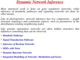
2. Introduction-Problem Statement • Problem proposed by Ruye Wang from Harvey Mudd College. • Some biological processes are modeled by networks comprised of a group of interacting components such as genes in a gene regulatory network, neurons in the brain, or proteins. • Biologists want to know how the components of the network are related and how they interact to make predictions about the behavior of a biological system.

3. Introduction • Network Inference is an approach for modeling and analyzing networks composed of many interacting component units. That is, given a set of genes a biologist performs a series of experiments to test how the genes affect (excite or inhibit) one another and also determine the magnitude of that affect.

4. Introduction • There are several different mathematical models for network inference each with it’s own advantages and disadvantages. • One is the Boolean Network Model which simulates the components by a group of binary nodes interacting with each other that follow logical operations.

5. Introduction • Another is the Linear and Quasi-Linear models that assume the components are linearly or quasi-linearly related in the network. • Then there is the Differential Equation (DE) model that simulates the dynamics of the network by a system of differential equations. This is the model we studied.

6. Introduction • Given a set of n nodes (genes) in the network and a set of k data points taken over time the differential equation governing the dynamics of the network is: • rivi’(t) + λivi(t) = g[Σ Tim vm(t) + hi] Where (i=1,…,n and t=1,…m) • vi(t) is the observed data and the other parameters are unknown where ri is a time constant, λi is a scaling factor, Tim is a constant that describes how node m affects node i, and hi is a constant.

7. Introduction • The goal is to find estimates for the n by n matrix T, along with the other unknown parameters from the observed data Vi(t). • However an optimal search of a O(n2)-dimensional space must be conducted in order to find the parameters that minimize the error. This is very computationally expensive and can realistically be done for a network with only a small number of nodes.

8. Our first Attempt • rv’ + λv= g(X) • Try to find a relationship between r and λ to reduce parameters. r λ r = f(λ) λ

9. But How? • Given g(x), some s function with range (-1,1) • g(x)= ex -1 then g’(x) Є (0,1] ex+1 αЄ (-1,1) and βЄ (0,1] rv’ + λv = g(X) rv’’ + λv = g’(X) a b c d r λ α β =

10. Other Methods • Most existing methods requires a heuristic approach • Requires many assumptions and parallel programming • Other than heuristic methods, statistical methods are viable but not feasible for large numbers of genes

11. Bayesian Networks • Statistical approach for modeling gene networks • Treats each gene as a random variable • Joint distribution over all genes represents the cell states • Goal: estimate and study the structures of the distributions • http://www.cs.huji.ac.il/labs/compbio/ismb01/ismb01.pdf • http://www.cs.unm.edu/~patrik/networks/robust.pdf

12. To Name a Few • Boolean Networks: uses 0’s and 1’s to represent the excitation or not http://www.cs.ucdavis.edu/~filkov/classes/289a-W03/l10.pdf • Differential Equation Models: • Many unknown parameters and assumptions • Nonlinear models needs to be linearized • Computationally costly for large number of genes http://www.biochemsoctrans.org/bst/031/1519/bst0311519.htm

13. Simulated Annealing • 1. Let X := initial configuration • 2. Let E := Energy(X) • 3. Let i = random move from the Moveset • 4. Let Ei := Eval(move(X,i)) • 5. If E < Ei then X := move(X,i) • E := Ei • Else with some probability, • accept the move even though • things get worse: • X := move(X,i) • E := Ei • 6. Goto 3 unless we have reached t_max Allowable moves. Choosing this is key!

14. Algorithm: Choosing (τ,λ) The domain of g-1 is (-1,1)! This is where conditions for λ come in.

15. Algorithm: Solving for T and h i.e

16. Algorithm: Decreasing Cost Tm decreases with each iteration. The more iterations the less likely you make possible “bad moves” same for change in cost.

17. Possible Area of Improvement • If we had more time where would we focus? • Simulated Annealing is a good idea provided you move within your moveset intelligently. • Choosing the moveset is also important, for us g(x) helps restrict the domain of λ based on τ. How do you know the domain of τ. • Finding the derivative matrix can possibly be improved. • Recovering the data, solving the ODE. • Choosing the correct energy function. • Solving the system of algebraic equations.

18. Ideas for moving within Moveset Neighborhood of search must be small enough. • Recall the computations: • Might be better to check if λ0 lies within the range dictated by τ1, and compare C(λ0 , τ1) to C(λ0 , τ0).

19. When k is not big enough, i.e. when k<n; • One obvious way could be: • Once we interpolate to get vi (t); • We can get as many time observations as we need, i.e. we can make k as big as necessary.

20. Another way could be: • Again taking DE as the model; • We can reduce the number of nodes, i.e. get a smaller number of nodes • To get all unknowns ,,Tij, hi we need to have k=n+1 or bigger. If k<n, then eliminate (n-k-1) nodes. • It can result in a loss of important data, the way we do that is really important. Thinking of vi (t)’s as functions, it’s possible that all n of them are linearly independent.

21. Functional Data Analysis (FDA)(*) could be extremely helpful in this manner. The thing is, in biological applications, we usually have huge n(~10000), and FDA is extremely useful in dealing with big data samples. • (*) Ramsay, J. O. and Silverman, B.W. (2002) Applied functional data analysis : methods and case studies, Springer series in statistics, New York ; London : Springer • (*) Ramsay, J. O. and Silverman, B.W. (2005) Functional data analysis, 2nd ed., New York : Springer • Also available to view online through Claremont campus:http://site.ebrary.com/lib/claremont/docDetail.action?docID=5006429

22. Working with the DE model, one immediately notices that computational cost (O(n2)) is a major obstacle. As long as complexity of FDA is not as big as O(n2), at does not make things any worse. (Actually, even if O(n2) is fine).