Download

1 / 31
310 likes | 435 Views
Yield Binomial. Bond Option Pricing Using the Yield Binomial Methodology. AGENDA. Background South African Complexity with option model Problems with Black and Scholes Approach Binomial Methodology. Background. American Bond Options - some traders use Black & Scholes model

E N D
Bond Option Pricing Using the Yield Binomial Methodology
AGENDA • Background • South African Complexity with option model • Problems with Black and Scholes Approach • Binomial Methodology
Background • American Bond Options - some traders use Black & Scholes model • Adjust for early exercise by forcing the answer to equal at least intrinsic
South African Complexity with Option Model • Overseas bond options have a fixed strike price throughout the option • South African bond options trade with a strike yield • Thus the strike price changes throughout the life of the option
South African Complexity with Option Model • Difference between Clean Strike prices and strike yield:
Problems with Black and Scholes approach • Tends to under-price out of the money option • Mispricing is the worst for short-dated bonds • Adjusting the Black & Scholes value with the intrinsic value results in discontinuity in value. • This also results in a discontinuity in the Greeks.
Example (1) • Put option on R150 • Settlement date: 26 Sept 2002 • Maturity date: 1 Apr 200 • Riskfree rate until option maturity: 10% (continuous) • Strike yield: 11.5% (semi-annual) • The YTM (semi-annual) ranges from 11.5% to 12.97% • Nominal: R100
We are interested in the point where the bond option premium falls below intrinsic Example (2)
Example (3) • The premium falls below intrinsic at a YTM of ± 11.84% • We are also interested in the behaviour of delta around a YTM of 11.84%
Example (4) • To this end, we use a numerical delta, calculated as follows: • Delta = UBOP(i+1) – UBOP(i) AIP(i+1) – AIP(i) • UBOP stands for used bond option premium, and is equal to the intrinsic whenever the option premium falls below intrinsic • AIP is the all-in price of the bond at the option’s settlement date
Example (5) • Delta makes a jump at the 11.84% mark
Example (6) • If we were to extend the data points in the first graph, it would look more or less as follows:
Example (7) • The Black and Scholes model will use: • The bond option premium if it is larger than intrinsic • Intrinsic, wherever the option premium falls below it • This is illustrated by the red dots:
What is different about the yield binomial model? • Normal binomial model uses a binomial price tree • Yield binomial uses yields instead of prices
Normal binomial model Using Risk Neutral argument we get: • a = exp(rt) • u = exp[.sqrt(t)] • d = 1/u • p = a - d u - d
Normal binomial model Time 2 Time 0 Time 1 S22=S11u p S11=S0u p 1-p S21= S0 S0 S0 p 1-p S10=S0d 1-p S20=S10d
Normal binomial model • From an initial spot price S0, the spot price at time 1 may jump up with prob p, or down with prob 1-p. • In the event of an upward jump, the S1 = S0u • In the event of a downward jump, the S1 = S0d • The probability p stays the same throughout the whole tree.
Yield binomial model Time 0 Time 2 Time 1 Y22=FY2u2 Y11=FY1u Y21=FY2 FY1 Y0 p2 Y10=FY1d 1-p2 Y20=FY2d2 FP2 FP1
Yield binomial model • At each time step the forward yield FYi is calculated • Then the yields at each node are calculated • Take first time step: • Y11 and Y10 is calculated by • Y11 = FY1 * u and • Y10 = FY1 * d
Yield binomial model Time 0 Time 2 Time 1 P22=P(Y22) p2 P11=P(Y11) p1 1-p2 P21=P(Y21) FP1 =P(FY1) Y0 p2 1-p1 P10=P(Y10) P20=P(Y20) 1-p2 FP2 FP1
Yield binomial model • In this model, a forward price FPiis calculated at time step i from the yields just calculated • At each node i,j, a bond price BPi,jis calculated from the yield tree • Cumulative probabilities CPi,j: CP0,0 = 1 CPi,j = CPi,j.(1-pi) if j=0 = CPi-1,j-1.pi + CPi-1,j.(1-pi) if 1j i-1 = CPi-1,i-1.pi if j=i
Yield binomial model The relationships between the forward prices FPi, bond prices Bpi,jand probabilities piare given by: FP1 = p1.BP1,1 + (1-p1).BP1,0 FP2 = CP2,2.BP2,2 + CP2,1.BP2,1+ CP2,0.BP2,0 FPi = sum(cumprob(I,j) *price(I,j) from j =0 to i p(i) = price(i) – sum(cumprob(i-1,j) * price(i,j)/ sum(cumprob(i-1,j)* price(I,j+1) –price(i,j))
Binomial Methodology… • Option Tree: • Calculate the pay-off at each node at the end of the tree. • Work backwards through the tree. • Opt. Price = Dics * [Prob. Up(i) * Option Price Up + Prob. Down(i) * Option Price Down]
Binomial Methodology • Checks on the model: • Put call parity must hold • Volatility in tree must equal the input volatility
Binomial Methodology in summary Option Inputs: • Strike yield • Type of option (A/E) • Is the option a Call or a Put?
Greeks • Numerical estimates • Alternative method for Delta and Gamma: • Tweak the spot yield up and down. • Calculate the option value for these new spot yields. • Fit a second degree polynomial on these three points. • The first ad second derivatives provide the delta and gamma.
Binomial Methodology in Summary • Calculated parameters - Yield and Bond Tree: • Time to option expiry in years • Time step in years • Forward yield and prices at each level in tree using carry model • Up and down variables
Benefits of Binomial • Caters for early exercise • Smooth delta • Flexibility with volatility assumptions
Binomial Model • Number of time steps? • Not a huge value in having more than 50 steps • Useful to average n and n+1 times steps