Download
1 / 41
410 likes | 585 Views
Electromagnetic Theory 55:070. Professor Karl E. Lonngren [lonngren@eng.uiowa.edu] 4312 SC office hours: 12:30 – 1:15 MWF. Demonstration in 2005. 207 CC. TA: Qiao Hu 1313 SC qiao-hu@uiowa.edu.

E N D
Electromagnetic Theory55:070 Professor Karl E. Lonngren [lonngren@eng.uiowa.edu] 4312 SC office hours: 12:30 – 1:15 MWF
TA: Qiao Hu1313 SC qiao-hu@uiowa.edu Text: “Fundamentals of electromagnetics with MATLAB” 2nd edition/2nd printing SciTech Press Grading 2 exams @ 100 -------- 200 Final exam ---------------- 150 Homework ---------------- 50 Total ----------------------- 400 Arthur Andersen who was recently fired by the Enron Corp. will audit the scores and the addition. Work together?
Check the WebSite for this class regularly! -- MATLAB programs -- Old exams Assignments -- Homework solutions -- Scores and Grades
super bubbles colliding galaxies
Ames Ames black hole
This is what happens to someone who does not want to learn electromagnetic theory!
example • EM Theory • MATLAB & vectors • static em fields • mathematics & MATLAB • Maxwell’s equations • electromagnetic waves & MATLAB • transmission lines & MATLAB • radiation & antennas & MATLAB
This course will not be one of those! http://www.jsonline.com/story/index.aspx?id=641947
MATLAB • in the college computers • easy to use & learn • easy to produce 2-d & 3-d plots • ODE & PDE • integrate & differentiate • get pictures – “.m” files in 070 web page • more MATLAB information on the CD
>> MATLAB icon >> x = 1 x = 1 >> complex numbers >> y = 1+1j (or 1+ 1i) y = 1.0000 + 1.0000i >> z = x - y z = 0 - 1.0000i >> math
>> x = 1; SAVE SPACE TRICK “ ; “ • >> y = 2; • >> z = x * y; % multiply • >> z • z = • 2 • >> w = x / y; % divide • >> w • w = • 0.5000
a = 1ux + 2uy + 3uz b = 3ux + 2uy + 1uz c = a + b c = 4ux + 4uy + 4uz >> a = [1 2 3]; >> b = [3 2 1]; >> c = a + b; c = 4 4 4 vectors - addition
a = 1ux + 2uy + 3uz b = 3ux + 2uy + 1uz a • b = b • a = 3 + 4 + 3 = 10 >> a = [1 2 3]; >> b = [3 2 1]; >> c = dot(a,b) c = 10 vectors - dot product
d = cross (a,b) d = 0 0 1 e = cross (b, a) e = 0 0 -1 vectors - cross product a = 1ux + 0uy + 0uz ==> a = [1 0 0]; b = 0ux + 1uy + 0uz ==> b = [0 1 0];
z B - A A B y x |B - A| = norm(B -A)
In MATLAB • >>colormap(hot) or cool or • >>whitebg(‘black’) or ‘green’ or • “print screen” • “paint”
simple graph >> x = [1 2 3 4 5] x= 1 2 3 4 5 >> plot(x) >> xlabel(‘#’) >> ylabel(‘value’)
semicolon two values >>x=[1 2 3 4 5]; >>y=[5 4 3 2 1]; >>plot(x,y,’*’) >>xlabel(‘x’) >>ylabel(‘y’)
Add to the graph • clear;clf • x=0:.1:4*pi; • plot(sin(x),'linewidth',3) • hold on • plot(cos(x),'linewidth',3,'linestyle','--') • xlabel('x','fontsize',18) • ylabel('V','fontsize',18) • set(gca,'fontsize',18) • whitebg('black')
>>[x,y]=meshgrid(-1:.1:1,-2:.4:4); >>R=(x.^2+(y+1).^2).^.5; >>Z=(1./R); >>surf(x,y,Z) >>view( - 37.5+ 90, 30)
>>[x,y]=meshgrid(-2:.2:2,-2:.2:2); >>r1=(x.^2+(y-.5).^2).^.5; >>r2=(x.^2+(y+.5).^2).^.5; >>V=(1./r1)-(1./r2); >>mesh(x,y,V) >>view(-37.5-90,10) >>colormap(hot)
>>[ex,ey]=gradient(V,.2,.2); >>quiver(x,y,ex,ey) >>grid
Iterate labels Change styles customize graphs -subplots
There are ".m" files on the Web page for this class. -The figures and the examples in the text -Additional programs may be added on an irregular basis
Government regulation may be required such as stop signs, stoplights, etc.