Download
1 / 129
1.33k likes | 1.53k Views
Statistical Nuclear Reaction Modeling. DIF/DPTA/SPN/LMED. S.Hilaire. Understanding basic reaction mechanism between particles and nuclei. Astrophysical applications (Age of the Galaxy, element abundancies …). Existing or future nuclear reactors simulations.

E N D
Statistical Nuclear Reaction Modeling DIF/DPTA/SPN/LMED S.Hilaire
Understanding basic reaction mechanism between particles and nuclei Astrophysical applications (Age of the Galaxy, element abundancies …) Existing or future nuclear reactors simulations Medical applications, oil well lodging, wastes transmutation … Finite number of experimental data (price, safety or counting rates) Complete measurements restricted to low energies ( < 1 MeV) Nuclear data needs Nuclear data needed for But Predictive Nuclear models (codes) essential
Content • Why and for whom ? • How ? • Modern methods • Few realistic examples • Future developments
1st PART Why and for whom ?
Why and for whom ? • What does the final product look like ? • What does it contain ? • What is it used for ? • Why do we need to perform evaluations ?
Portion of a evaluated file (FORMAT ENDF) Content nature (s) Target mass Target identification (151Sm) Values Content type (n,2n) Number of values Material number
Content of an evaluated file • General Informations (authors, method used, date, version, etc …) • Resonances parameters • Cross sections - Integrated, spectra and angular distribution, doubly differential - (n,f), (n,g), (n,n’), (n,p), (n,d), …, (n,2n), …,(n,2na), (n,pa), ………. • Decay schemes • Multiplicities • Uncertainties, Covariance data
What is it used for ? • Produce nuclear data libraries • (ENDF, CENDL, BROND, JENDL, JEFF) • Feed codes with evaluated nuclear «constants» • Non-proliferation and lugage scan • Nuclear power plants (classical or new generation) • Electronic damage (space) • Radiotherapy • Geology (oil well logging, …) • Non-destructive control • Fuel cycle, waste management …
Why do we need data evaluations ? Problems due to microscopic data • Too few or no experimental data • Incoherent experimental informations Evaluated files problems • Bad description of integral experiment • Bad evaluations or only partial
CRITICAL SPHERE Atomic composition 239Pu 73.8 % 240Pu 19.4 % 241Pu 3.00 % 242Pu 0.40 % Ga 3.40 % Geometry M = 19.46 0.156 Kg r = 15.73 g/cm3 R = 6.66 cm K effectif 1.00000 0.002 Bad description of integral experiment Benchmark JEZEBEL 240Pu SIMULATION Caractéristiques code MCNP4C2 110 cycles de 2000 particules librairie BRC6 pour le 239Pu Résultats BRC6 1.00086 0.00135 ENDF/B6.7 1.00016 0.00138 JEFF3 1.00400 0.00131 JENDL3.3 1.00341 0.00110
2nd PART How ?
How ? • Experimental data interpolation • Bayesian methods • Renormalisations of existing evaluations • Copy/Paste of other evaluations • Nuclear reaction modeling
___ ___ ___ (n,n’cont) (n,2n) (n,p) Cross section (barns) Energy (MeV) Experimental data interpolation 58Ni (JEFF 3.0)
Bayesian methods • Method : Account for new experimental data to improve an existing evaluation without re-doing everything. Suppress crazy data points. • Advantages : Provides variances & covariances simultaneously with the new evaluation. Perfect agreement with the available experimental points. • Drawbacks : A large quantity of experimental points are required. Depends on the choice of the « prior »
Renormalized to fit a given set of experimental points JENDL-3.2 original Renormalisations
Expertise. Cut and Paste Á new evaluation can be restricted (only specific cross section are given) or only a given energy range is covered (ex: E > 1keV ). A complete evaluation is obtained by copiing selected parts from other evaluations correctly chosen
Parameter Libraries Nuclear Reaction Modeling Method which consists in using a physical model (together with sets of parameters) to calculate evaluated data. Evaluated Data Physical Model Parameters Observables Experimental Data
3rd PART Nuclear Reaction Modeling
Nuclear Reaction Modeling • Models sequence • Optical model and direct reactions • Pre-equilibrium model • Compound Nucleus model • Fission • Level densities • Neutron multiplicities • Uncertainties
Compound Nucleus Direct components Pre-equilibrium Reaction time d2s / dWdE Emission energy
Direct (shape) elastic Elastic Reaction NC Fission OPTICAL MODEL COMPOUND NUCLEUS PRE-EQUILIBRIUM Tlj Inelastic (n,n’), (n,), (n,), etc… Direct components Models sequence
Angular distributions Integrated cross sections Transmission coefficients Optical model This model yields :
Direct interaction of a projectile with a target nucleus considered as a whole Quantum model Schrödinger equation U Complex potential: U = V + iW Refraction Absorption Optical Model
Phenomenologic Microscopic Adjusted parameters Weak predictive power Very precise ( 1%) Important work No adjustable parameters Usable without exp. data Less precise ( 5-10 %) Quasi-automated Total cross sections Two types of approaches
Total cross section (barn) Neutron energy (MeV) Phenomenologic optical model • 20 adjusted parameters • Very precise (1%) • Weak predictive power
[ ] U(r,E) = VV(E)f(r, RV,aV) +VS(E) g(r,RS,aS) [ ] + i WV(E)f(r,RV,aV) + WS(E)g(r,RS,aS) -1 f(r,R,a)= 1+exp((r-R)/a) g(r,R,a) = - df/dr Phenomenologic optical model U(r,E) = U(r,E) = V(E,r) + i W(E,r) Well depths (MeV) Incident energy (MeV)
OMP & Its parameters Resolution of the Schrödinger equation Calculated observables sel-inl (q), Ay(q), stot, sreac, S0,S1 sReaction, Tlj, sdirect Phenomenologic optical model Experimental data sel-inl(q), Ay(q), stot, sreac , S0,S1
Semi-microscopic optical model • No adjustable parameters • Based on nuclear structure properties usable for any nucleus • Less precise than the • phenomenological approach
Effective Interaction U(r(r’),E) = Optical potential Radial densities r(r’) = r(r) U(r,E) = Independent of the nucleus Depends on the nucleus Depends on the nucleus Semi-microscopic optical model
(n,n) , (p,p) et (p,n) Semi-microscopic optical model Unique description of elastic scattering
Semi-microscopic optical model Enables to perform predictions for very exotic nuclei for which There exist no experimental data
14 MeV 184W(n,n’) 744 keV 6+ 364 keV 4+ 112 keV 2+ 0+ b 0 { 184W (T+V00-E) Y0 = V02Y2 (T+V22-E) Y2 = V20Y0 Impact of coupled channels
Sections efficaces (mb) Impact of coupled channels
Result without any coupling Impact of coupled channels experiment Spectrum (barn.MeV-1) Emission energy (MeV)
Shape elastic Elastic Reaction NC Fission OPTICAL MODEL COMPOUND NUCLEUS PRE-EQUILIBRIUM Tlj Inelastic (n,n’), (n,), (n,), etc… Direct components Models sequence
E 0 EF 1p 2p-1h 3p-2h 4p-3h time time 1n 3n 5n 7n Pre-equilibrium model Compound Nucleus
dP(n,E,t) = dt S teq sc (E, ec) dec = sR P(n, E, t) l n, c(E) dt dec n, Dn=2 0 Pre-equilibrium model(Exciton model) P(n,E,t) = Probabilité to find for a given time t the composite system with an energy E and an excitonsnumber n. Probability l a, b (E) = Transition rate from an initial state a towards a state b for a given energy E. Evolution equation P(n-2, E, t) l n-2, n(E) +P(n+2, E, t) l n+2, n(E) Apparition [ ] l n, n+2(E) + l n, n-2(E) + l n, emiss(E) - P(n, E, t) Disparition Emission cross section in channel c
Cross section Outgoing energy 9% 45% 79% 39% 16% 12% <ETot>= 12.1 <EDir>= 24.3 <EPE>= 9.32 <ESta>= 2.5 (MeV) Pre-equilibrium model Total Direct Pre-equilibrium Statistical 39%
Pre-equilibrium model 14 MeV neutron + 93 Nb without pre-equilibrium without pre-equilibrium (barn) d/dE(b/MeV) pre-equilibrium Compound nucleus Outgoin neutron energy (MeV) Iincident neutron energy (MeV)
Shape elastic Elastic Reaction NC Fission OPTICAL MODEL COMPOUND NUCLEUS PRE-EQUILIBRIUM Tlj Inelastic (n,n’), (n,), (n,), etc… Direct components Models sequence
+ NC N’’,Z’’,E’’*,J’’ N’,Z’,E’*,J’ N,Z,E*,J r(N’’,Z’’,E’’*) r(N’,Z’,E’*) r(N,Z,E*) Compound nucleus model After direct and pre-equilibrium emission dir + pre-equ reaction = N0 Z0 E*0 J0 N0-dND Z0-dZD E*0-dE*D J0-dJD N0-dND-dNPE Z0-dZD-dZPE E*0-dE*D-dE*PE J0-dJD-dJPE = E = Z = E* = J E Z E* J …
Compound nucleus model ab = p p Tb Pb= 2 2 ka ka STc c (CN)=Ta a (CN)Pb a TaTb ab = STc c Compound nucleus hypothesys • Continuum of excited levels • Independence between incoming channel a and outgoing channel b Hauser- Feshbach formula
Compound nucleus model Channel Definition a + A (CN )*b+B Incident channel a = (la, ja=la+sa, JA,pA, EA, Ea) • Conservation equations • Total energy : Ea + EA = ECN = Eb + EB • Total momentum : pa + pA = pCN = pb + pB • Total angular momentum : la + sa + JA = JCN = lb + sb + JB • Total parity : pA (-1) = pCN = pB (-1) lb la
Compound nucleus model p S S p = J=| IA–sa | S (2J+1) J+IA ja+sa J+IB jb +sb S S S S c (2IA+1) (2sa+1) ja=| J–IA | la=| ja–sa | jb=| J–IB| lb=| jb –sb| TJp W IA +sa+la max a,la, ja, b, lb, jb dp (a) dp (b) TJp TJp T T ka TJp 2 b, lb, jb a, la , ja T c, lc , jc In realistic calculations, all possible quantum number combinations have to be considered sab =