Download

1 / 13
130 likes | 317 Views
CONSUMER BEHAVIOR AND UTILITY MAXIMIZATION Pertemuan 17. Matakuliah : J0114-Teori Ekonomi Tahun : 2009. Law of Diminishing Marginal Utility. Terminology Utility is the benefit or satisfaction a person receives from consuming a good or a services

E N D
CONSUMER BEHAVIOR AND UTILITY MAXIMIZATIONPertemuan 17 Matakuliah : J0114-Teori Ekonomi Tahun : 2009
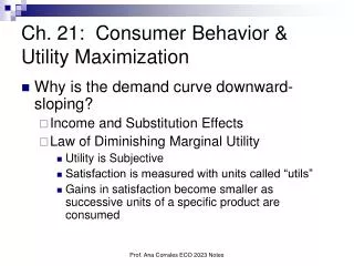
Law of Diminishing Marginal Utility • Terminology • Utilityisthe benefit or satisfaction a person receives from consuming a good or a services • Total Utility is total amount of of satisfaction or pleasure a person derives from consuming some specific • Marginal Utility is the extra satisfaction aconsumer realizes from and additional unit of that product
30 20 ] ] ] ] ] ] ] 10 0 1 1 2 2 3 3 4 4 5 5 6 6 7 7 10 8 6 4 2 0 -2 Law of Diminishing Marginal Utility Total Utility TR (1) Tacos Consumed Per Meal (2) Total Utility, Utils (3) Marginal Utility, Utils Total Utility (Utils) 0 10 18 24 28 30 30 28 0 1 2 3 4 5 6 7 10 8 6 4 2 0 -2 Units Consumed Per Meal Marginal Utility Marginal Utility (Utils) MU Units Consumed Per Meal
Theory of Consumer Behavior • Consumer Choice and Budget Constraint • Rational Behavior • Preferences • Budget Constraint • Prices • Utility Maximizing Rule • Allocate Money Income so that Last Dollar Spent on Each Product Yields the Same Marginal Utility
(3) Product B: Price = $2 Theory of Consumer Behavior Numerical Example: Utility-Maximizing Combination of Products A and B Obtainable with an Income of $10 (2) Product A: Price = $1 (b) Marginal Utility Per Dollar (MU/Price) (b) Marginal Utility Per Dollar (MU/Price) (a) Marginal Utility, Utils (a) Marginal Utility, Utils (1) Unit of Product First Second Third Fourth Fifth Sixth Seventh 10 10 10 10 12 8 8 24 18 9 7 7 8 16 Final Result – At These Prices, Purchase 2 of Item A and4 of B
8 Utils 16 Utils $1 $2 Theory of Consumer Behavior Algebraic Restatement: MU of Product A MU of Product B = Price of B Price of A = Optimum Achieved - Money Income is Allocated so that the Last Dollar Spent on Each Product Yields the Same Extra or Marginal Utility
Deriving the Demand Curve Same Numeric Example: 2 Quantity Demanded Price Per Unit of B Price of Product B $2 4 1 1 6 Income Effects Substitution Effects DB 0 4 6 Quantity Demanded of B
O 19.3 Applications and Extensions • DVDs and DVD Players • The Diamond-Water Paradox • The Value of Time • Medical Care Purchases • Cash and Noncash Gifts
12 10 8 Quantity of A 6 4 2 0 2 4 6 8 10 12 Income = $12 Quantity of B PA= $1.50 Income = $12 PB= $1 Indifference Curve Analysis • Budget Line (Constraint) • Income Changes • Price Changes Total Expenditure Units of A (Price = $1.50) Units of B (Price = $1) (Unattainable) 8 6 4 2 0 0 3 6 9 12 $12 12 12 12 12 (Attainable)
12 10 8 Quantity of A 6 4 2 0 2 4 6 8 10 12 Quantity of B Indifference Curve Analysis • What is Preferred • Downsloping • Convex to Origin • Marginal Rate of Substitution (MRS) j Combination Units of A Units of B j k l m 12 6 4 3 2 4 6 8 k l m I
MRS = 12 10 8 Quantity of A 6 4 PB 2 PA 0 2 4 6 8 10 12 Quantity of B Indifference Curve Analysis • The Indifference Map • Equilibrium Position at Tangency Preferred – But Requires More Income W X I4 I3 I2 I1
12 Marginal Utility of B Marginal Utility of A 10 = 8 Price of B Price of A 6 Quantity of A 4 X 2 I3 I2 0 2 4 6 8 10 12 Quantity of B $1.50 1.00 .50 Derivation of the Demand Curve • Measurement of Utility At $1 Price for B, 6 Units are Purchased Record the Results As Price of B Increases to $1.50, Only 3 Units of B are Bought Record the Results Connect the Points to Create the Demand Curve Price of B DB 1 2 3 4 5 6 7 8 9 10 11 12 Quantity of B