Download
1 / 17
190 likes | 528 Views
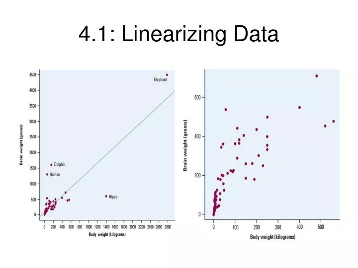
4.1: Linearizing Data. Logs of both sides: Linearized. Which model for prediction should you choose?. Plot the data and look for patterns. Is there a linear pattern? Use Ch. 3. If no to #1: try exponential model. If no to #2, try power function model.

E N D
Which model for prediction should you choose? Plot the data and look for patterns. • Is there a linear pattern? Use Ch. 3. • If no to #1: try exponential model. • If no to #2, try power function model. • If no to #3, check for a dimensional relationship. • If no to #4, try the hierarchy of powers.
Example: Linearizing Curved Data“Playing” with the data in order to linearize it
#4.1, 4.2: Classwork 4.1 Hint L1 = length, L2 = weight, L3 = cube-root of L2 4.2Hint L1=length, L2 = period, L3 = square root of L1
Steps to transform data • Transform (linearize) the data (exponential? Log the y’s; Power? Log both the x’s and the y’s) • Perform regression (check r, r-squared) and write new equation (with a and b) • Make residual plot (check that it’s a good model) • Perform an inverse transformation to get the model for the original data.
Ratio Test • To see if a set of data with a consistent increment in the x-values is growing exponentially, we calculate the ratios of y-values to previous y-values. • If these quotients are approximately the same, then the points are increasing (quotient >1) or decreasing (quotient <1) exponentially.
Example 4.5 Gordon Moore predicted that the number of transistors on an integrated circuit chip would double every 18 months. Here’s the actual data:
Calculator Tip for Ratio Test • Copy the y values (in L2) into L3. • Since we want to calculate y2/y1, delete the first number in L3. • Since L2 and L3 need to be the same length, delete the last number in L2. • Define L4=L3/L2. These are the ratios you want.
If our data is growing exponentially and we plot the log of y against x, we should observe a straight line for the transformed data.
The table shows the federal debt (in trillions) for the years 1980 through 1991. • Construct a scatter plot. Perform an appropriate test to decide whether the data is exponential or not. Show the common ratios. • Calculate the logarithms of the y-values and extend the table above to show the transformed data Then perform least-squares regression on the transformed data. Write the LSRL equation for the transformed data. • What is the correlation coefficient? • Is this correlation between YEAR and FEDERAL DEBT? Explain briefly. • Now transform your linear equation back to obtain a model for the original federal debt data. Write the equation of this model. • Compare and comment on your models prediction for 1990 and 1991 to the actual federal debt. • Use your model to predict the national debt in the year 2000. • Would you use this model to predict future debts? Why/why not?