Download
1 / 23
230 likes | 327 Views
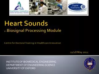
David A. Clifton, W.K. Kellogg Junior Research Fellow Institute of Biomedical Engineering University of Oxford. Fourier analysis Biomedical Signal Processing Centre for Doctoral Training in Healthcare Innovation davidc@robots.ox.ac.uk. Fourier analysis.

E N D
David A. Clifton, W.K. Kellogg Junior Research Fellow Institute of Biomedical Engineering University of Oxford Fourier analysisBiomedical Signal ProcessingCentre for Doctoral Training in Healthcare Innovationdavidc@robots.ox.ac.uk
Fourier analysis Introduction to Fourier analysis, the Fourier series Sampling and Aliasing Discrete Fourier methods, and Applications
2: Sampling, Aliasing, and Spectra Amplitude modulation Sampling Recovering a signal after sampling Aliasing Anti-aliasing
Amplitude Modulation Amplitude modulation means to modulate the amplitude of some carrier wave according to some interesting signal: E.g., a high-frequency sinusoidal carrier wave injected through a patient’s chest might be modulated by their respiration The envelope of the result then corresponds to the interesting signal (here, respiration)
Amplitude Modulation f(t) xg(t) F(ω) *G(ω) Amplitude modulation is merely the multiplication of one signal g(t) (the carrier) by some other signal f(t) (the information wave) We have previously seen that if we multiply in the time domain, this corresponds to convolution in the frequency domain: ...where we generally try to avoid convolution, primarily because it is terrifying:
Amplitude Modulation f(t) xg(t) F(ω) *G(ω) And yet we can avoid all of the convolution difficulties. Recall that our information signal f(t) is being multiplied by a sinusoidal carrier wave g(t) We saw previously that the FT of a sinusoid was just a delta function: ...so multiplying f(t) by a sinusoidal wave is the same asconvolving with a delta function
Amplitude Modulation f(t) xg(t) F(ω) *G(ω) f(t) x cos(ω0t) F(ω) *π[δ(ω±ω0)] Happily, convolving with a delta function is the one special case of convolution that we can easily handle: ...because convolving with a delta function δ(ω±ω0) just does the following to F(ω):
Amplitude Modulation We could recover our original information from the modulated signal using demodulation, which just selects the relevant frequency information (using a filter) ...and we can then recover our original time-signal using FT-1 (Hence the term modem: modulation-demodulation)
Sampling The concept of amplitude modulation is very useful, and employed whenever we wish to turn continuous signals (such as those we measure from patients) into discrete quantities that can be manipulated by computers: digitisation, a.k.a. sampling Whenever we sample, we multiply our original signal by a sampling function, p(t):
Sampling That’s my pulse train What is the sampling function, p(t)? ...a.k.a. a train of pulses / Dirac deltas
Sampling I was the Lucasian Professor of Mathematics at a certain minor university, a position latterly held by Stephen Hawkin The FT of p(t) is: We know what happens to F(ω) when we convolve it with δ(ω±ωs)... This time, we’re convolving F(ω) with δ(ω) , δ(ω±ωs) ,δ(ω±2ωs), etc.
Sampling Convolving F(ω) with δ(ω) , δ(ω±ωs) ,δ(ω±2ωs), has the following effect: ...where the frequency spectrum of our interesting signal f(t) is repeated at multiples (harmonics!) of the sampling frequency
Sampling (This is a reconstruction filter) Just as we previously recovered our original signal after amplitude modulation, we can pick out our original signal after sampling using a filter: ...allowing us to recover our time-series by performing FT-1, as before
Sampling problems Sufficiently high ωs: Insufficiently high ωs: What could possibly go wrong with this idyllic situation? If the sampling frequency ωs is too low, the images of the frequency spectrum begin to overlap, termed aliasing
Problem 1: aliasing Information Theory was mine, btw. Hej, I’m actually Swedish [NIK-VIST] Use of our reconstruction filter would include components from higher- and lower- frequency images, hence we would not obtain the original signal: Aliasing can be avoided if ωs > 2 ωm(the Nyquist-Shannon theorem)
Problem 1: aliasing fs < 2 fm fs < 2 fm fs = fm The corresponding behaviour in the time domain is obvious is we consider a sinusoid of frequency fm : Hence we have to sample at least twice every period in order to disambiguate, and so fs > 2 fm, or equivalently ωs > 2 ωm
Problem 2: non-bandlimited signals Our previous signal was very well-behaved, in that its frequency spectrum F(ω)was limited to a certain band of frequencies – this made it easy to separate from its images that appear after sampling. It was band-limited. However, most signals are not so well-behaved, and contain a wide spread of frequencies. We need to decide the highestfrequency of interest in F(ω),and then suppress all higher frequencies using ananti-aliasingfilter
Problem 2: non-bandlimited signals We then sample the anti-aliased signal, which produces non-overlapped (unaliased) images in the frequency domain:
Problem 2: non-bandlimited signals Finally, we can apply our reconstruction filter to pick out the original signal, after sampling: but this leads to potential problem #3...
Problem 3: non-ideal filters Sadly, real filters are not ideal – they are not “brick wall” filters, and have some “roll-off” slope If the filter is a low order, some components from the images will once again appear in the window – further aliasing! Thus, the less ideal the filter, the greater the sampling frequency must be in order to adequately separate the images
We now know that... • Amplitude modulation results in: • Sampling, which is a form ofamplitude modulation, results in: • Aliasing can be avoided by: • A sampling rate > than the Nyquist-Shannon frequency • Using an anti-aliasing filter to band-limit our signal • Understanding that our reconstruction filter is non-ideal
Warning • Sampling allows us to represent our continuous time-domain signal using discrete pulses... • ...but the corresponding frequency spectrum remains continuous! • For analysis in a computer, we need to be able to store the frequency spectrum in a discrete form. • We need the Discrete Fourier Transform.
David A. Clifton, W.K. Kellogg Junior Research Fellow Institute of Biomedical Engineering University of Oxford Fourier analysisBiomedical Signal ProcessingCentre for Doctoral Training in Healthcare Innovationdavidc@robots.ox.ac.uk