Download
1 / 18
180 likes | 242 Views
Explore the spatial distribution of antiprotons in the magnetosphere with computational models, revealing their origins and trajectories in relation to cosmic rays and Earth's magnetic fields.

E N D
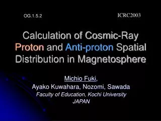
ECRS2004 Aug.31-Sep.3 Cosmic-Ray Antiproton Spatial Distributions Simulatedin Magnetosphere Abstract:The recent balloon experiments as well as satellites and space-station experiments have been demonstrated the flux and the energy spectrum of antiprotons which naturally exist around the earth. Specially they are observed on the top of atmosphere in the polar region and believed to be secondarily produced from the high energy cosmic-ray interactions with interstellar matter. They have the characteristic energy around 2 GeV and are influenced with the Earth's magnetic fields. I computed the motion of antiprotons in the Magnetosphere region with some initial conditions and plotted the spatial distributions of them. The antiprotons in the polar region are looked like coming from the outer region. Meanwhile, the antiprotons in the space-station region are trapped in the radiation belts. The source of the former may be the produced particles from the collisions of Cosmic-rays on the Sun surface or in the extra-solar region. The latter is explained by the model that antiprotons are originated in decay particles from the antineutrons produced with the cosmic ray interactions in atmosphere. They gather in the radiation belts as well as protons and electrons. The plots show that in the space-station altitudes they are rich in the SAA region. In order to distinguish between antiprotons and protons effectively, the differences of arrival directions of them are important. Michio Fuki Faculty of Education, Kochi University 2-5-1, Akebono-cho, Kochi 780-8520, JAPAN
1. Motivation • 1-1 Experiments of anti-proton observation • Balloon experiments ⇒ antiprotons &protons • Satellites/Space-station ⇒ protons, nuclei, electrons) • BESS, CAPRICE, etc. • AMS, HEAT, PAMERA… • Where and How much natural anti-protons exist around the Earth ? • Computer simulation estimates the spatial and energy distributions, to make clear the antiproton origin.
1) Energy Spectrum ●Protons●Anti-protons(< 1/10000) Fisk BESS Mode energy ~0.3 – 0.7 GeV Mode energy ~ 2.0 GeV
2)Radiation spatial distribution (Alt.400km) Where anti-protons? ●Proton & electron(by Mir) ●Neutron(RRMD@STS) Solar-min Solar-max Abundant in SAA and both magnetic poles
2. Computation model 2-1 Equation of Motion Lorentz force F; m: mass , c :light velocity,q:charge, V :velocity, B:magnetic field (static), ⇒Magnetosphere(IGRF) E = 0;⇒ no electric field
2-2Injection models(Initial conditions) Protons • I) protons(free injection out of magnetosphere) galactic (or solar) cosmic ray primary protons :GCR • II) p + A → p + X (nuclear collision with atmosphere) creation@20 km, Albedo protons :CRAP • III)p + A → n + X (nuclear collision with atmosphere) n → p + e- + ν (decay from albedo neutron) τ = 900sec, creation<10・RE, decayed protons :CRAND Antiprotons, (collision origin;pair creation) • I) galactic cosmic ray antiprotons (similar to protons) • II) p + A → p + p+ p-+ X(pair-creation) • III)p + A → p + n + n-+ X(pair-creation) n-→ p- + e+ + ν (decay from anti-neutrons)
Three injection models for protons GCR CRAP CRAND
Anti-proton Energy Spectra from Monte Carlo Simulation ・Accelerator data and simulation ・Simulation in lab. system 200 100 50 GeV Eo= 20 10 5 GeV Multi-Chain-model for p-A collision, each 100,000 events
2.3 Energy spectrum form Analytical form Monte Carlo form
Kinetic energy spectral function (Model-Ⅰ&Ⅱ) • Em: mode energy, a, b: spectral power index • set a = -1, b = 2.0. • Em = 0.3 GeV for protons(solar minimum era), • Em = 2.0 GeV for antiprotons. • Decayed proton/antiproton spectra(Model-Ⅲ) (anti)neutron decay-time:τ= 900sec,yield time t = 0.2sec.
3. Computing method and parameters Solve 3D equation of motion(1) numerically by time • Adamus-Bashforth-Moulton 6th method used • (better than Runge-Kutta-Gill 4th method) • Range:RE(=6,350km)+20km ~ 10・RE(in magnetosphere) • Time step:variable,10 μsec(<1000km)~ 10 msec(outer) • Time limit: trace up to max.600sec(10 min.) • Magnetosphre fields: static, IGRF (inner region) + Mead (outer region) Use Monte Carlo simulation for initial conditions • Energy range:10 MeV ~ 10 GeV random • Sample from Energy spectrum • Starting position and direction: random(uniform, isotropic) • (Anti)neutron decay:random(τ=900 sec),< 10・RE
4. Results: Spatial distribution(1) ModelⅡ CRAP モデル-II ModelⅠ GCR ModelⅢ CRAND モデル-III Input 100,000 protons
・) Surface distribution in Polar region@400km Protons/Model-I input 100,000 particles Aurora zone Antiprotons/Model-I input 100,000 particles Wide spread Spatial distribution (2)
・) World surface distribution onISS @400km Protons/Model-III Input 100,000 particles East tail Antiprotons/Model-III Input 100,000 particles West tail Looks gathering in SAA Spatial distribution (3) Same color means same particle (orbits)
Altitude distribution cross section (Φ=-50deg(SAA) and 130deg(opposite side) ) ●Protons●Antiprotons Spatial distribution(4) Proton rich around 4000 km and antiprotons rich in 2000 km Low altitude components → SAA
Differences of arrival directions between protons and anti-protons ISS@400km ●Protons Input 100,000 particles from above: north east from below: south east ● Antiprotons Input 100,000 particles from above: south west from below: north west
4. Conclusions • Polar region (High latitude) • Cosmic-ray (anti)protons arrive to both polar regions (by modelⅠ)・・・・due to Rigidity Cut-off • Antiprotons is more spread than protons in polar regions • Radiation belts • Decayed (anti)protons make Van-Allen radiation belts (CRAND; Cosmic ray Albedo neutron decay:modelⅢ) • Low energy(<0.1GeV)decayed protons are trapped widely • High energy(~1GeV)antiprotons are trapped in inner zone • Antiprotons are gathered in low altitudes (~2000km) • at ISS altitudes • Protons and antiprotons are same gathered in SAA region • Arrival directions are opposite for protons (north east) and antiprotons (south west) • Tails of protons are east, tails of antiprotons are west (These are qualitative)
5. Discussions and future subjects • Spatial distribution of protons and antiprotons are simulated qualitatively • More statistics! • 100K partilcles→1M…..now,10K/1day(Pentium4,2.4GHz) • Needs quantitative discussion by unified model: • Flux, p-/p-ratio, (nuclei, isotope, anti-helium?) • Energy spectrum, Direction distribution. • Production rate,Trapping time,Leakage rate. • Time fluctuation (short,long). • Solar activity, Modulations etc. • Needs comparisonwith other results • Theory・Simulation • (coming)Experimental data • Other solar effects • magnetic fields, of Sun, Planets