Data Analysis

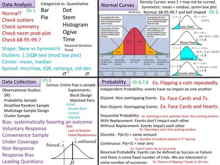
1. Density Curves: area 1 + may not be curved. Symmetric: mean = median, symm box plot Normal: 68-95-99.7 and bell shaped Data Analysis Categorical vs. Quantitative Bar Dot Pie Stem Histogram Ogive Time Normal Curves Ch 1 Ch 2 Normal? Check outliers Check symmetry Check norm prob plot Check 68-95-99.7 Less than More than Seasonal Variation Trend Shape: Skew vs Symmetric Outliers: 1.5IQR test (mod box plot) Center: mean, median Spread: min/max, IQR, variance, stddev Interval Double Sided Ch 5 Data Collection Probability Ch 6,7,8 Ex. Flipping a coin repeatedly. Census: Entire Pop is sample Observational Studies: Experiments: SRS Block Design Probability Sample Matched Pairs Stratified Random Sample Multistage Sample Design Cluster Sample Independent Probability: events have no impact on one another Disjoint: Non overlapping Events Non Disjoint: Overlapping Events Sequential Probability: With Replacement: Events don’t impact each other Without Replacement: Events impact each other Discrete: P(x=5) = some amount Continuous: P(x=5) = near zero Binomial Probability: Events can be defined as Success or Failure and there is some fixed number of trials. We are interested in some number of successes. Ex. Face Cards and 7s. Good: Double Blind Control Placebo Bad: Lack of Realism Failed Randomness Ex. Face Cards and Hearts. Ex. Selecting a card, putting it back, then picking another. Bias: systematically favoring an outcome Voluntary Response Convenience Sample Under Coverage Non Response Response Bias Leading Questions Ex. Selecting a card, then picking another. Ex. Number of students absent in 2nd period. Ex. Time it takes me to run a mile. Ex. Chance of flipping 7 heads in 10 tries.

2. Inferences! Ch 2 This wouldn’t make sense.. Individuals can’t be proportions… Use this to find the percentile an individual is in. n = 1 Use Table A For z-scores Ch 10 Same as below since we use Z-scores with proportions as long as both rules of thumb are met and the sample is a SRS from the population of interest. Use Table A for z-scores Ch 11 Ch 12 Use Table B for t-scores Interpreting Hypothesis Tests Pooled: Interpreting Confidence Intervals Why pool? “We are C% confident the true mean is between the lower and upperbound.” “If we gathered many sample means, C% of the resulting intervals would contain the true mean.”

3. 2 Way Tables Chi-Squared Tests Ch 4 Ch 13 Goodness of Fit Conditional Probability “On the condition that somebody is old, what is the probability that they smoke?” 9 / 31 Marginal Distributions Homogeneity “What percent of participants were smokers?” 18 / 87 “What percent were old?” 31 / 87 Simpson’s Paradox: Seemingly paradoxical event where a data set is divided up into 2 data sets based on some condition and those 2 data sets favor 1 analysis while the original data set favors a contradictory analysis. Least Squares Ch 3 Inference and Regression Ch 14 Comparing two lists of values: x and y How to interpret: Direction: positive or negative Form: linear, exponential (x v. log y), or power (log x v. log y) Strength: 0 to 1 (weak, moderate, strong) Numeric Summary: Causation: We cannot make conclusions about causation Common Response: Some other variable (z) is having a causal impact on both x and y. Confounding Variables: Variable x has a casual impact on y but some other variable (z) is also having a causal impact on y. X and Z are competing. Hypothesis Testing Confidence Intervals