Download
1 / 34
340 likes | 371 Views
Explore the historical basis, principles & applications of probability theory, learn about probability models, distributions & inference methods, including examples and techniques for making predictions.

E N D
Bases of the theory of probability and mathematical statistics.
History • Games of chance: 300 BC • 1565: first formalizations • 1654: Fermat & Pascal, conditional probability • Reverend Bayes: 1750’s • 1950: Kolmogorov: axiomatic approach • Objectivists vs subjectivists • (frequentists vs Bayesians) • Frequentist build one model • Bayesians use all possible models, with priors
Concerns • Future: what is the likelihood that a student will get a CS job given his grades? • Current: what is the likelihood that a person has cancer given his symptoms? • Past: what is the likelihood that Marilyn Monroe committed suicide? • Combining evidence. • Always: Representation & Inference
Basic Idea • Attach degrees of belief to proposition. • Theorem: Probability theory is the best way to do this. • if someone does it differently you can play a game with him and win his money. • Unlike logic, probability theory is non-monotonic. • Additional evidence can lower or raise belief in a proposition.
Probability Models: Basic Questions • What are they? • Analogous to constraint models, with probabilities on each table entry • How can we use them to make inferences? • Probability theory • How does new evidence change inferences • Non-monotonic problem solved • How can we acquire them? • Experts for model structure, hill-climbing for parameters
Discrete Probability Model • Set of RandomVariables V1,V2,…Vn • Each RV has a discrete set of values • Joint probability known or computable • For all vi in domain(Vi), Prob(V1=v1,V2=v2,..Vn=vn) is known, non-negative, and sums to 1.
Random Variable • Intuition: A variable whose values belongs to a known set of values, the domain. • Math: non-negative function on a domain (called the sample space) whose sum is 1. • Boolean RV: John has a cavity. • cavity domain ={true,false} • Discrete RV: Weather Condition • wc domain= {snowy, rainy, cloudy, sunny}. • Continuous RV: John’s height • john’s height domain = { positive real number}
Cross-Product RV • If X is RV with values x1,..xn and • Y is RV with values y1,..ym, then • Z = X x Y is a RV with n*m values <x1,y1>…<xn,ym> • This will be very useful! • This does not mean P(X,Y) = P(X)*P(Y).
Discrete Probability Distribution • If a discrete RV X has values v1,…vn, then a prob distribution for X is non-negative real valued function p such that: sum p(vi) = 1. • This is just a (normalized) histogram. • Example: a coin is flipped 10 times and heads occur 6 times. • What is best probability model to predict this result? • Biased coin model: prob head = .6, trials = 10
From Model to PredictionUse Math or Simulation • Math: X = number of heads in 10 flips • P(X = 0) = .4^10 • P(X = 1) = 10* .6*.4^9 • P(X = 2) = Comb(10,2)*.6^2*.4^8 etc • Where Comb(n,m) = n!/ (n-m)!* m!. • Simulation: Do many times: flip coin (p = .6) 10 times, record heads. • Math is exact, but sometimes too hard. • Computation is inexact and expensive, but doable
Learning Model: Hill Climbing • Theoretically it can be shown that p = .6 is best model. • Without theory, pick a random p value and simulate. Now try a larger and a smaller p value. • Maximize P(Data|Model). Get model which gives highest probability to the data. • This approach extends to more complicated models (variables, parameters).
Another Data Set What’s going on?
Mixture Model • Data generated from two simple models • coin1 prob = .8 of heads • coin2 prob = .1 of heads • With prob .5 pick coin 1 or coin 2 and flip. • Model has more parameters • Experts are supposed to supply the model. • Use data to estimate the parameters.
Continuous Probability • RV X has values in R, then a prob distribution for X is a non-negative real-valued function p such that the integral of p over R is 1. (called prob density function) • Standard distributions are uniform, normal or gaussian, poisson, etc. • May resort to empirical if can’t compute analytically. I.E. Use histogram.
Joint Probability: full knowledge • If X and Y are discrete RVs, then the prob distribution for X x Y is called the joint prob distribution. • Let x be in domain of X, y in domain of Y. • If P(X=x,Y=y) = P(X=x)*P(Y=y) for every x and y, then X and Y are independent. • Standard Shorthand: P(X,Y)=P(X)*P(Y), which means exactly the statement above.
Marginalization • Given the joint probability for X and Y, you can compute everything. • Joint probability to individual probabilities. • P(X =x) is sum P(X=x and Y=y) over all y • Conditioning is similar: • P(X=x) = sum P(X=x|Y=y)*P(Y=y)
Marginalization Example • Compute Prob(X is healthy) from • P(X healthy & X tests positive) = .1 • P(X healthy & X tests neg) = .8 • P(X healthy) = .1 + .8 = .9 • P(flush) = P(heart flush)+P(spade flush)+ P(diamond flush)+ P(club flush)
Conditional Probability • P(X=x | Y=y) = P(X=x, Y=y)/P(Y=y). • Intuition: use simple examples • 1 card hand X = value card, Y = suit card P( X= ace | Y= heart) = 1/13 also P( X=ace , Y=heart) = 1/52 P(Y=heart) = 1 / 4 P( X=ace, Y= heart)/P(Y =heart) = 1/13.
Formula • Shorthand: P(X|Y) = P(X,Y)/P(Y). • Product Rule: P(X,Y) = P(X |Y) * P(Y) • Bayes Rule: • P(X|Y) = P(Y|X) *P(X)/P(Y). • Remember the abbreviations.
Conditional Example • P(A = 0) = .7 • P(A = 1) = .3 P(A,B) = P(B,A) P(B,A)= P(B|A)*P(A) P(A,B) = P(A|B)*P(B) P(A|B) = P(B|A)*P(A)/P(B)
Note Joint yields everything • Via marginalization • P(A = 0) = P(A=0,B=0)+P(A=0,B=1)= • .14+.56 = .7 • P(B=0) = P(B=0,A=0)+P(B=0,A=1) = • .14+.27 = .41
Simulation • Given prob for A and prob for B given A • First, choose value for A, according to prob • Now use conditional table to choose value for B with correct probability. • That constructs one world. • Repeats lots of times and count number of times A= 0 & B = 0, A=0 & B= 1, etc. • Turn counts into probabilities.
Consequences of Bayes Rules • P(X|Y,Z) = P(Y,Z |X)*P(X)/P(Y,Z). proof: Treat Y&Z as new product RV U P(X|U) =P(U|X)*P(X)/P(U) by bayes • P(X1,X2,X3) =P(X3|X1,X2)*P(X1,X2) = P(X3|X1,X2)*P(X2|X1)*P(X1) or • P(X1,X2,X3) =P(X1)*P(X2|X1)*P(X3|X1,X2). • Note: These equations make no assumptions! • Last equation is called the Chain or Product Rule • Can pick the any ordering of variables.
Extensions of P(A) +P(~A) = 1 • P(X|Y) + P(~X|Y) = 1 • Semantic Argument • conditional just restricts worlds • Syntactic Argument: lhs equals • P(X,Y)/P(Y) + P(~X,Y)/P(Y) = • (P(X,Y) + P(~X,Y))/P(Y) = (marginalization) • P(Y)/P(Y) = 1.
Bayes Rule Example • Meningitis causes stiff neck (.5). • P(s|m) = 0.5 • Prior prob of meningitis = 1/50,000. • p(m)= 1/50,000 = .00002 • Prior prob of stick neck ( 1/20). • p(s) = 1/20. • Does patient have meningitis? • p(m|s) = p(s|m)*p(m)/p(s) = 0.0002. • Is this reasonable? p(s|m)/p(s) = change=10
Bayes Rule: multiple symptoms • Given symptoms s1,s2,..sn, what estimate probability of Disease D. • P(D|s1,s2…sn) = P(D,s1,..sn)/P(s1,s2..sn). • If each symptom is boolean, need tables of size 2^n. ex. breast cancer data has 73 features per patient. 2^73 is too big. • Approximate!
Notation: max arg • Conceptual definition, not operational • Max arg f(x) is a value of x that maximizes f(x). • MaxArg Prob(X = 6 heads | prob heads) yields prob(heads) = .6
Idiot or Naïve Bayes: First learning Algorithm Goal: max arg P(D| s1..sn) over all Diseases = max arg P(s1,..sn|D)*P(D)/ P(s1,..sn) = max arg P(s1,..sn|D)*P(D) (why?) ~ max arg P(s1|D)*P(s2|D)…P(sn|D)*P(D). • Assumes conditional independence. • enough data to estimate • Not necessary to get prob right: only order. • Pretty good but Bayes Nets do it better.
Chain Rule and Markov Models • Recall P(X1, X2, …Xn) = P(X1)*P(X2|X1)*…P(Xn| X1,X2,..Xn-1). • If X1, X2, etc are values at time points 1, 2.. and if Xn only depends on k previous times, then this is a markov model of order k. • MMO: Independent of time • P(X1,…Xn) = P(X1)*P(X2)..*P(Xn)
Markov Models • MM1: depends only on previous time • P(X1,…Xn)= P(X1)*P(X2|X1)*…P(Xn|Xn-1). • May also be used for approximating probabilities. Much simpler to estimate. • MM2: depends on previous 2 times • P(X1,X2,..Xn)= P(X1,X2)*P(X3|X1,X2) etc
Common DNA application • Looking for needles: surprising frequency? • Goal:Compute P(gataag) given lots of data • MM0 = P(g)*P(a)*P(t)*P(a)*P(a)*P(g). • MM1 = P(g)*P(a|g)*P(t|a)*P(a|a)*P(g|a). • MM2 = P(ga)*P(t|ga)*P(a|ta)*P(g|aa). • Note: each approximation requires less data and less computation time.