Download

1 / 39
390 likes | 409 Views
This talk discusses the impact of processes in the subtropical marine boundary layer on cloud structure and coverage, and the challenges in representing them in numerical models. It presents an integrated approach to estimate MBL depth, decoupling, and entrainment using observations and reanalysis data.

E N D
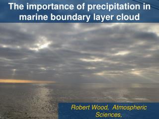
Boundary layer depth, entrainment, decoupling and clouds over the eastern Pacific Ocean Robert Wood, Atmospheric Sciences, University of Washington
Motivation • Processes in the subtropical MBL have enormous impact upon the structure and coverage of clouds which strongly impact the earth’s radiation budget • The depth of the MBL has a marked impact upon its dynamics and structure - measurements are sparse • MBL structure and the clouds therein are poorly represented in large scale numerical models
Organization of this talk • The structure of the subtropical MBL • Clouds and the subtropical MBL • MBL depth and decoupling estimates using integrated approach • Entrainment estimates….and further
SST anomaly from zonal mean ERBE net cloud forcing
Subtropical ocean winds McNoldy et al. (2004)
Tropical-subtropical general circulation from Randall et al., J. Atmos. Sci., 37, 125-130, 1980
Riehl et al. (1951) Inversion base
First map of MBL depth (1961) 1400 m 1600 m 1800 m 600 m 2000 m 1000 m 1200 m Hawaii Neiburger (1961)
qv qv The structure of the subtropical MBL • MBL is deeper over warmer water • Deeper MBLs show two-layer structure decoupling the cloud layer from the surface from Albrecht et al., JGR, 100, 14209-14222, 1995
free troposphere mixed layer Well mixed layer from Stevens et al., QJRMS, 129, 3469-3493, 2003
Decoupled MBL free troposphere (FT) cloud layer subcloud layer surface mixed layer from Nicholls and Leighton, QJRMS, 112, 431-460, 1986
Clouds and the subtropical MBL qv qv composite profiles from Albrecht et al., JGR, 100, 14209-14222, 1995
How well do various BL mixing schemes perform? Observations (ERBE) stratocumulus trade cumulus
This study • Integrative approach to estimate MBL properties in regions of low cloud • Combines observations from MODIS and TMI with reanalysis from NCEP and climatology from COADS • Results in estimates of MBL depth and decoupling (and climatology of entrainment)
MBL model • “PLR” model - Park, Leovy and Rozendaal: A New Heuristic Lagrangian Marine Boundary Layer Cloud Model. J. Atmos. Sci.,61, 3002–3024, 2004 • Tweak on a mixing-line model to describe the boundary layer structure • First applied to MBL by Betts (1982) • Describes mixing between surface and free-tropospheric air
Conserved variables • Under moist adiabatic processes, we use: (1) liquid potential temperature: L (1 - LvqL/cpT) (2) total water content: qT=qv+qL [whereqLand qv the liquid water and water vapor mixing ratios]
Mixing line model? • Air at some level in the MBL is a mixture of surface and free-tropospheric (FT) air • Any variable C conserved under moist adiabatic processes: C(z) = [1-(z)]C(0) + (z)C(FT) where (z) [0,1] is independent of C =1 if air is entirely from FT, =0 if entirely from surface • Key is how to specify the function (z)
zi=1685 m z/zi=1.15 zi=715 m z/zi=0.2 Mixing line? observations from Albrecht et al., JGR, 100, 14209-14222, 1995
Decoupling parameters C(z) = [1-(z)]C(0) + (z)C(FT) Consider C(z)=C(zi-), i.e. at the inversion base, with C(FT)=C(zi+), i.e. above the inversion C(zi-) = [1-(zi-)]C(0) + (zi-)C(zi+) Rearrange as C(zi-) = C(0) + (zi-)[C(zi+)-C(0)] where we define = (zi-) =0 for well-mixed MBL, =1 for MBL without an inversion. Real MBLs somewhere in between
Model profile structure used arbitrary profile shape LCL
Methodology • Decoupling parameters are related: = q[1-0.2CF] • Independent observables: LWP, SST - Ttop • Unknowns: zi,q • Use climatological surface RH and air-sea temperature difference • Reanalysis free-tropospheric temperature and moisture • Iterative solution employed to resulting non-linear equation for zi and q
Datasets • NASA MODIS (Moderate Resolution Imaging Spectro-radiometer) – cloud LWP, cloud top temperature Ttop • all available daytime data from Terra satellite, Sept-Oct 2000 (almost complete daily coverage at 10:30 local hr) • swath data split into analysis “scenes” of 256x256 km • TMI (TRMM microwave imager) – SST • use 3-day composites from Wentz, www.remss.com • NCEP/NCAR reanalysis– free tropospheric boundary conditions (T, qv at 700 hPa, and later ws) • interpolate 6 hourly data at 2.5o resolution to nearest MODIS “scene”
Mean MBL depth (Sep/Oct 2000) NE Pacific SE Pacific
Mean decoupling parameter q Decoupling scales well with MBL depth
Composite LWC profile estimates from SF to Hawaii [g m-3] mean zi mean zcb mean zML Hawaii SF
Relationship between MBL depth and cloud fraction from Wood and Hartmann 2005, submitted to J. Climate.
Relationship between MBL depth and mesoscale cellular convection (MCC) increasing zi from Wood and Hartmann 2005, submitted to J. Climate.
Deriving mean entrainment rates WHY? • Use equation: we = uzi+ws • Estimate wsusing NCEP reanalysis • Estimateuziusing NCEP winds (interpolated to zi) and two month mean zi The entrainment rate is a key parameter which determines the rate at which free tropospheric air is incorporated into the MBL HOW?
Mean entrainment rates Entrainment rate [mm s-1]◄ NE PacificSE Pacific ►Subsidence rate [mm s-1]
Summary • Presented new method to estimate both MBL depth and decoupling using an integration of satellite observations and a simple MBL model • Over most of the subtropical regions studied the MBL is decoupled to some extent and that the decoupling becomes more pronounced as the MBL deepens • Cloudiness and mesoscale variability found to be strongly correlated with MBL depth, suggesting that MBL depth is a key variable in the Sc-Cu transition • Mean entrainment rates were derived. Together with the zi estimates these provide strong constraints for numerical models.
Future directions • Expanding analysis over longer timescales and different regions • Use results to constrain GCM parameterizations and other models of MBL and cloud processes • Examine whether observed decoupling is consistent with theory of decoupling for non-precipitating MBLs – is drizzle necessary to drive decoupling in the subtropical MBL?
tropical-subtropical general circulation from Randall et al., J. Atmos. Sci., 37, 125-130, 1980
Physics of the ScCu transition • When the subcloud buoyancy flux (TKE production rate) < 0 results from LES models (e.g. Stevens 2000) show that mixed layer theory is violated and MBL tends to develop a two layer structure with the upper (cloud) layer being partially isolated from the moisture source • Mixed layer theory can be used to predict the limits of its own validity using the subcloud buoyancy flux (e.g. Bretherton and Wyant 1997)
Physics of the ScCu transition 2 • Bretherton and Wyant (1997) use a minimal mixed layer model to derive a “decoupling” criterion: LHF > (zi/hAent)R where LHF is the surface latent heat flux, R is the radiative flux loss from the MBL,h is the cloud thickness, and Aent is the entrainment efficiency (we=Aentw*3/b) • Recent work suggests Aent ≈ 1.2 for cloud topped BLs. • R ≈ 40 W m-2for subtropical cloudy boundary layers (diurnal average) • LHF from COADS, ziandhfrom this analysis