Download
1 / 60
600 likes | 783 Views
Scalable localized routing in wireless sensor networks. Tutorial. Ivan Stojmenovic Ivan@site.uottawa.ca www.site.uottawa.ca/~ivan. Sensors route reports to a fixed sink …. Internet. humidity. Sink. End user. Multi-hop networks: Routing. Unit graphs radius. Sensor networks

E N D
Scalable localized routing in wireless sensor networks Tutorial Ivan Stojmenovic Ivan@site.uottawa.ca www.site.uottawa.ca/~ivan Ivan Stojmenovic
Sensors route reports to a fixed sink … Internet humidity Sink End user Ivan Stojmenovic
Multi-hop networks: Routing Unit graphs radius Sensor networks Position information • Routing: source destination Ivan Stojmenovic
Routing with/out position information ? • Sensors can function efficiently only with position informationGPS and location estimation advanced rapidly(cubic cm sensor with 7mm x 7mm x 2mm GPS) • Sink can flood network with/out its own position • Routes can be learn while flooding, or • Only position of sink is learned and used Ivan Stojmenovic
Proactive routing: ad hoc networks • Routing table contains the first hop/neighbor toward each destination • Bellman-Ford: Each node exchanges its routing tables with all its neighbors, and • Best neighbors N for route from S to D is one that minimizes: cost of link S to N + cost N to D (from routing table in N) • OLSR (Optimized Link State Routing): link changes are flooded + Dijkstra’s shortest path • MPR (MultiPoint Relay) to reduce flooding Ivan Stojmenovic
Reactive routing: ad hoc networks • Source floods route discovery (short) message • Destination node replies back to source upon receiving discovery message(s) using memorized hops (AODV) or paths (DSR) • Source sends full message using recorded path • Multi-paths for QoS • Route discovery message may contain accumulated delay, congestion, power, cost etc. along paths; best path selected at destination • Local route maintenance; expanding ring search Ivan Stojmenovic
S D S D Route discovery by flooding Each sensor retransmits once Problem: sink stable but sensors may sleep DSR, AODV in ad hoc networks, position info not needed = ‘directed diffusion’ for sensors Intanagonwiawat, Govindan, Estrin 2000 Ivan Stojmenovic
Directed diffusion • Monitoring center broadcasts packet to all sensors in a region • Sensors create links for reporting along reverse broadcast tree • Link is toward sensor from which the first copy of packet is received Ivan Stojmenovic
Greedy position based localized routing A D S B Localized protocol: S knows only position of itself, its neighbors and destination D S forwards to neighbor B closest to D Finn 1987 Ivan Stojmenovic
Greedy: SABCD vs shortest path SECD S A D B C E Localized vs. globalized protocol SP Overhead: messages to maintain global information at each node following mobility and/or sleep/active periods changes Ivan Stojmenovic
Greedy is loop-free An A1 A2 An-1 D A3 Assume A1 closest to D A2 sends to A3 – contradiction, A1is closer Ivan Stojmenovic
Progress based routing ‘84-86. A B C A’ D S E F MFR: Choose closest projection on SD; minimize SA.SD Ivan Stojmenovic
MFR is loop-free An A1 A2 An-1 D A3 A1 A2 Proof by Stojmenovic, Lin 1998 Ivan Stojmenovic
Greedy vs. MFR B A S D A’ B’ may choose different node AD<BD choice is same most of time! Similar performance Ivan Stojmenovic
DIRectional routing methods Basagni, Chlamtac, Syrotiuk, Woodward MOBICOM’98 (DREAM) Ko, Vaidya MOBICOM ’98 (LAR) Kranakis, Singh, Urrutia CCCG’99 (compass routing) A D S Closest direction Send to allneighbors within angular range from direction [BCSW,KV] location update schemes [BCSW, KV] Flooding rate (# of messages vs SP) ?? Ivan Stojmenovic
DIR is not loop-free ! E H D F G Transmission radius Stojmenovic 1998 Greedy and MFR are loop free Ivan Stojmenovic
Performance evaluation • Random unit graphs: Choose n nodes at random in [0,m]x[0,m] • select average node degreed = 2,3,4,5,… • sort all (n-1)n/2 edges in increasing order • Radius R= nd/2-th edge in sorted order! • Reject graph if disconnected Success rate = high for high degree, low for low degree hop count = successful Greedy/MFR close to SP, DIR > floodingrate (#messages vs SP) = close to SP Independent variable is d, not R !!! Ivan Stojmenovic
Is hop count the best metric ? • Power consumption • Reluctance (avoiding nodes with low energy) • Power_reluctance • Delay • Expected hop count (realistic physical layer) • COST - selected metric Ivan Stojmenovic
Cost to progress ratio framework • Progress: measures advance toward destination • Progress = |SD|-|AD|=d-a • Select neighbor A that minimizes cost(SA)/progress(A) • Hop count: cost=1 • Maximize advance A a r Stojmenovic IEEE Network 2006 D S d Ivan Stojmenovic
Parameterless behavior • Cost-to-progress ratio framework has no added parameters such as thresholds • Threshold based approach: eliminate ‘bad’ links, drop packet if there is no ‘good’ neighbor • What if a solid path has just one weak ‘bridge’? • Experiments so far indicate that threshold based approaches are inferior for all threshold values - either high failure rate or suboptimal since there is no notion of ‘best’ neighbor Ivan Stojmenovic
Power saving localized routing A d B Constant power minimize hop count power =u(d)= d + c minimize total power Many articles assume c=0; in practice c>0 since power is needed to run hardware at each node, and correct reception requires minimal transmission power (no energy free transmission at zero distance) reluctance f(A) to forward packets = =1/g(A) g(A) in [0,1] lifetime minimize total cost Power_reluctance= f(A)u(d) model by Rodoplu, Meng 1999 Ivan Stojmenovic
A s r S x A d-x D D S d Ideal and localized power aware routing • # of hops nd(a( -1)/c)1/ • minimal power: v(d)=dc(a(-1)/c)1/ + da(a( -1)/c)(1-)/= O(d) • A = minimizes u(r)+ v(s) among neighbors of S Stojmenovic, Lin 1998 Ivan Stojmenovic
Localized power aware routing A a r D S d • Kuruvila, Nayak, Stojmenovic 2004 • Power progress:minimize (r+c)/(d-a) • Iterative power progress: select B if power(SB)+power(BA) < power(SA) • (Iterative) Projection power progress Ivan Stojmenovic
‘Reluctance’ routing algorithm a r D d S Stojmenovic, Lin 1998 Rediscovered by: Yu, Govindan, Estrin: GEAR, TR-01-0023, Aug. 2001. A f(A)= reluctance =1/g(A) g(A) in [0,1] lifetime A = neighbors of S that minimizes f(A) + f’(S)*s/R ( cost of A + average cost around S * ideal number of hops from A to D) If D is neighbor of S then deliver to D else forward to A Reluctance/progress: minimize f(A)/(|SD|-|SA|) Kuruvila, Nayak, Stojmenovic 2004(no added parameters) Ivan Stojmenovic
Power_reluctance routing A a r D d S Stojmenovic, Lin 1998 A = neighbors of S that minimizes u(r) + v(s) If D is neighbor of S and u(d) < min [u(r) + v(s)] then deliver to D else {A = neighbor of S that minimizes f(A)u(r) + v(s)f’(S); forward to A } Power*reluctance/progress: minimize f(A)power(SA)/(|SD|-|SA|) Kuruvila, Nayak, Stojmenovic 2004(no added parameters) Ivan Stojmenovic
A a r D d S Physical layer impact • Expected hop count (counting all transmissions and possibly acknowledgements) • F(SA)= expected hop count from S to A • Minimize F(SA)/(d-a) • Kuruvila, Nayak, Stojmenovic 2004 • Delay … • QoS routing … • Bitrate … Ivan Stojmenovic
Physical layer impact Lognormal shadowing model • =4 p(R)=0.5 Packet reception probability Unit graph model: Prp(x)=1, xR Prp(x)=0, x>R R Distance between nodes What is the transmission radius ? Who are neighbors? Ivan Stojmenovic
Simulation dilemma • Home-made simulator or one used by others (NS-2, Qualnet, J-sim,…)? • Greedy routing uses hop count as measure • NS-2 applies realistic physical layer, which mostly penalizes long hops • Why to use simulator that defeats the model, hides physical models and parameters which impact the data, impact comparison, and provide no explanation? • Solution: build protocols and simulators in parallel, so that results can be explained and protocols improved • Network layer protocol need to be designed with more realistic physical layer, not with unit disk graph model Ivan Stojmenovic
How to simulate ? • Study one variable at a time, explain it fully • Ideal MAC, no congestion, for initial studies • If one routing A is on average better than one routing B, it should cause less congestion, thus show even more advantage at the transport layer • Simulation to match ‘ideal’ assumptions • Stable graphs first; localized design takes care of dynamics • Independent variable is one that matters e.g. density (average number of neighbors per node), not transmission radius • Compare against the best (e.g. shortest path), not against worst (e.g. flooding) Ivan Stojmenovic
Approximate packet reception probability p(x) 1-(x/R)q/2 for x < R (2-x/R)q/2 for 2R x R q depends on L, packet length, 2 6 • Signal strength is a random variable, and deviation cannot be predicted in advance (but some articles use it to select best neighbors) • Transmission power is assumed fixed and same • q=1 for L=1; q2 for L=120. • Exact formula complex, time consuming and unreliable • each bit is received or not independently (no coding) packet received correctly iff all bits received Ivan Stojmenovic
Reactive routing with physical layer • In route discovery phase, forward the sum of Expected Hop Counts along partial route, or • Wait retransmission proportional to EHC on link • Problems: • A single retransmission by a given node may not reach the best forwarding neighbor; tradeoff # of retransmissions and gains made • Real traffic may not use routes created by control traffic – different packet lengths, or low packet reception probability Ivan Stojmenovic
Hello messages with physical layer • ‘fixed hello protocol’ • Send hello messages fixed number of times, to increase the probability of reception by neighbors • ‘variable hello protocol’ • Send hello packets until sufficient number of such packets from neighbors received (learn enough neighbors for desired density) • Goel, Kalaichelvan, Nayak, Stojmenovic, Villanueva-Pena 2006 Ivan Stojmenovic
Greedy routing is not hop count optimal x x x x x x 1 n x = d/n d • Ideal routing • Place additional nodes between Source and Destination as required. • Ideal Hop count computed for different u and values • Each received packet is acknowledged u times • Low values for 0.6Rx 0.9R u=1 • 50% higher at x=R, very high x>R or x<0.1R • Kuruvila, Nayak, Stojmenovic 2004 Ivan Stojmenovic
IHC for Different u Values (=2) Ivan Stojmenovic
Expected progress routing a x A c D Hop by hop ack C Progress: c-a Expected hop count for u=1: f(x,1) = 1/p2(x)+1/p(x) Best value of u: u1/p(x) Forward to neighbor (closer to destination) that maximizes (c-a)/f(x,1) (EPR-1) or (c-a)/f(x,u) (EPR-u) Ivan Stojmenovic
tR Greedy Algorithm • The redefined notion of greedy routing. • Current node S selects neighbor closest to D among all neighbors that are closer to D than itself, and which are at distance at most tR from S, for forwarding the message. • Experiments for t = 1, 1.25 and 1.4377 • Threshold based greedy routing Ivan Stojmenovic
Performance summary • Good performance for localized parameterless algorithms • low hop counts for dense networks and 100% success rates • tR-greedy are significantly inferior: a choice of ‘long’ edge is quite likely on a route which then contributes to very high expected hop count measure, or • ‘optimistic’ parameter choice fails traffic unnecessarily Ivan Stojmenovic
Loop-free with guaranteed delivery • Stop if message is to be returned to neighbor it came from = concave node • MFR, DIR, Greedy • FloodingGreedy, Flooding MFR: • Concave nodes flood message to all neighbors and then reject further copies of the same message • Loop-free methods that guarantee delivery, reasonable flooding rate • But nodes memorize past traffic Stojmenovic, Lin 1999 Ivan Stojmenovic
D Routing around void areas ? A ? S Recovery, perimeter, face mode Ivan Stojmenovic
1. Constructing planar graph: faces Bose, Morin, Stojmenovic, Urrutia, 1999 D A ? S Some planar graphs (Gabriel graph) can be constructed without message exchange! Ivan Stojmenovic
2. Traverse proper face until recovery Bose, Morin, Stojmenovic, Urrutia, 1999 D S ? B • Select face containing SD • Follow that face by left hand or right hand rule • until recovery (= closer node reached) C Ivan Stojmenovic
GFG= Greedy-FACE-Greedy • run Greedy until delivery or a failure node A, |AD|=d, • run FACE until delivery or B reached, |BD|<d, • run Greedy … • paths close to SP for higher degrees, • <3.5 times longer than SP for low degrees • No traffic memorization, localized, close to SP scalable !! • Karp and Kung MOBICOM 2000 duplicated (with citation) GPSR= GFG (added MAC, mobile nodes) Bose, Morin, Stojmenovic, Urrutia, 1999 Ivan Stojmenovic
Gabriel graph P Q W V U Gabriel, Sokal 1984 Gabriel graph GG(S) contains an edge (U,V) iff the disk with diameter (U,V) contains no other point from S = distance from other points to center of UV is > |UV|/2 = Acute angles for all joint neighbors in GG GG(S) is planar and connected (contains MST) Ivan Stojmenovic
Gabriel graph is planar Planar graph = no two edges intersect Proof by contradiction: Assume UV, PQ GG(S), UV PQ P U Q V PUQ < /2, PVQ < /2, • UPV < /2, UQV < /2, Sum of angles in UPVQ < 2 Ivan Stojmenovic
Gabriel graph contains MST P Q W By contradiction: Assume PQ MST, PQ GG; W, PW<PQ, QW<PQ, PWMST Replace PQ by PW in MST new MST has smaller sum of edge lengths. contradiction Gabriel graph connected Ivan Stojmenovic
Unit (connected) graph contains MST Kruskal’s algorithm to construct MST: Sort all edges by their length, from shortest to longest. Consider each edge in that order for inclusion in MST: Include it in MST if its addition does not create a cycle. Unit graph edges considered before any other edge. After their consideration, MST is already connected, and no more edges can be added. GG(S) U(S) planar and connected! Ivan Stojmenovic
Traversal of selected face leads to recovery D E X S ? F B C • Line SD intersects the face in X on an edge EF • E or F is closer to D than A (if nothing else found before) Ivan Stojmenovic
S X D F Getting closer on the face is guaranteed for GG E S < /2, D< /2 since EF is in GG E > /2 or F > /2 F > /2 |SD| > |FD| F is closer to D than S Frey, Stojmenovic MOBICOM 2006 Ivan Stojmenovic
Conclusions • Imprecise location information is challenge for georouting with guaranteed delivery • Georouting in 3D has no guaranteed delivery • Unit disk graph is required • For planar graphs GFG still always works, but GPSR by Karp and Kung does not • For other metrics, there is still no alternative to GG based face routing for recovery mode, which prefers close neighbors (except shortcuts, dominating sets..) Frey, Stojmenovic 2006 Ivan Stojmenovic
Greedy, GFG (greedy-face-greedy) J G U K L D A V F W B I E C H Ivan Stojmenovic