Download
1 / 19
190 likes | 332 Views
Computing a tree. Genome 559: Introduction to Statistical and Computational Genomics Prof. James H. Thomas. time. Defining what a “tree” means. unrooted tree (used when the root isn’t known):. rooted tree (all real trees are rooted):. sequences (leaves or tips). branch points. root.

E N D
Computing a tree Genome 559: Introduction to Statistical and Computational Genomics Prof. James H. Thomas
time Defining what a “tree” means unrooted tree (used when the root isn’t known): rooted tree (all real trees are rooted): sequences (leaves or tips) branch points root ancestral sequence branches time vaguely radiates out from somewhere near the center …divergence time is the sum of (horizontal) branch lengths
A tree has topology and distances Are these different trees? Topologically, these are the SAME tree. In general, two trees are the same if they can be inter-converted by branch rotations.
The number of tree topologies grows extremely fast 3 leaves 3 branches 1 internal node 1 topology (3 insertions) 4 leaves 5 branches 2 internal nodes 3 topologies (x3) (5 insertions) In general, an unrooted tree with N leaves has: 2N – 3 branches N – 2 internal nodes ~ O(N!) topologies 5 leaves 7 branches 3 internal nodes 15 topologies (x5) (7 insertions)
There are many rooted trees for each unrooted tree For each unrooted tree, there are 2N - 3 times as many rooted trees, where N is the number of leaves (# internal branches = 2N – 3). 20 leaves - 564,480,989,588,730,591,336,960,000,000 topologies
How can you compute a tree? Many methods available, we will talk about: Distance trees Parsimony trees Others include: Maximum-likelihood trees Bayesian trees
Distance tree methods • Measure pairwise distance between each pair of sequences. • Use a clustering method to build up a tree, starting with the closest pair.
Distance matrix from alignment (symmetrical, lower left not filled in)
Distance matrix methods • Methods based on a set of pairwise sequence distances, typically from a multiple alignment. • Try to build the tree that best matches the distances. • Usual standard for “best match” is the least squares of the tree distances compared to the real pairwise distances: Let Dm be the real distances and Dtbe the tree distances. Find the tree that minimizes:
Enumerate and score all trees • Enumerate every tree topology, fit least-squares best distances for each topology, keep best. • Not used for distance trees - there is a much faster way to get very close to correct. • Called Neighbor-Joining algorithm, one of a general class called hierarchical clustering algorithms.
Sequential clustering approach (UPGMA) 1 2 5 3 4
Sequential clustering algorithm generate a table of pairwise sequence distances and assign each sequence to a list of N tree nodes. look through the current list of nodes (initially these will all be leaf “nodes”) for the pair with the smallest distance. merge the closest pair, remove the pair of nodes from the list and add the merged node to the list. repeat until there is only one node left - it is the root. (in words, this is the arithmetic average of the distances between all the leaves in one node and all the leaves in the other node)
Neighbor-Joining Algorithm (side note) Essentially as for UPGMA, but correction for distance to other leaves is made. Specifically, for sets of leaves iand j, we denote the set of all other leaves as L, and the size of that set as , and we compute the corrected distance Dij as: (the mean distance from i to all 'other' leaves)
Data structure for a tree class TreeNode: <parent node> <left-child node> <right-child node> <distance to parent> The tree itself is made up of TreeNode objects, each of which is connected to other TreeNode objects based on its three attributes. How do we know a node is a leaf? A root? A leaf (or tip) has no child nodes. A root has no parent node. All the rest have all three.
Raw distance correction • As two DNA sequences diverge, it is easy to see that their maximum raw distance is ~0.75 (assuming equal nt frequencies). • This graph shows evolutionary distance related to raw distance: DNA
Mutational models for DNA • Jukes-Cantor (JC) - all mutations equally likely. • Kimura 2-parameter (K2P) - transitions and transversions have separate rates. • Generalized Time Reversible (GTR) - all changes may have separate rates. (Models similar to GTR are also available for protein)
Jukes-Cantor purines pyrimidines Kimura 2-parameter
Jukes-Cantor model - distance correction Jukes-Cantor model: Draw is the raw distance (what we directly measure) D is the corrected distance (what we want) ln is natural log Similar calculations can be made for the other models (but more complex).
Distance trees - summary • Convert each pairwise raw distance to a corrected distance. • Build tree as before (UPGMA or neighbor-joining). • Notice that these methods do not consider all tree topologies - they are very fast, even for large trees.