Download
1 / 12
120 likes | 255 Views
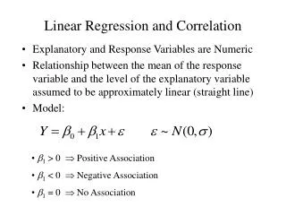
CHAPTER 12. Linear Regression and Correlation. Example. The table shows the math achievement test scores for a random sample of n = 10 college freshmen, along with their final calculus grades. Example. The ANOVA Table. The Calculus Example:. Least squares regression line.

E N D
CHAPTER 12 Linear Regression and Correlation
Example The table shows the math achievement test scores for a random sample of n = 10 college freshmen, along with their final calculus grades.
Least squares regression line Regression Analysis: y versus x The regression equation is y = 40.8 + 0.766 x Predictor Coef SE Coef T P Constant 40.784 8.507 4.79 0.001 x 0.7656 0.1750 4.38 0.002 S = 8.70363 R-Sq = 70.5% R-Sq(adj) = 66.8% Analysis of Variance Source DF SS MS F P Regression 1 1450.0 1450.0 19.14 0.002 Residual Error 8 606.0 75.8 Total 9 2056.0 Regression coefficients, a and b Minitab Output
Measuring the Strength of the Relationship • If the independent variable x is useful in predicting y, you will want to know how well the model fits. • The strength of the relationship between x and y can be measured using:
Measuring the Strength of the Relationship • Since Total SS = SSR + SSE, r2 measures • the proportion of the total variation in the responses that can be explained by using the independent variable x in the model. • the percent reduction in the total variation by using the regression equation rather than just using the sample mean y-bar to estimate y.
Interpreting a Significant Regression • Even if you do not reject the null hypothesis that the slope of the line equals 0, it does not necessarily mean that y and x are unrelated. • Type IIerror—falsely declaring that the slope is 0 and that x and y are unrelated. • It may happen that y and x are perfectly related in a nonlinear way.
Some Cautions • You may have fit the wrong model. • Extrapolation—predicting values of y outside the range of the fitted data. • Causality—Do not conclude that x causes y. There may be an unknown variable at work!
Example The table shows the heights (in cm) and weights(in Kg) of n = 10 randomly selected college football players.