Download
1 / 21
230 likes | 528 Views
Introduction to Econometrics. Lecture2 Bivariate regression models Interpreting least squares regression results: goodness of fit and significance tests Forecasting with a simple regression model. Recommended reading. DOUGHERTY Introduction to Econometrics Chapter 2 OR

E N D
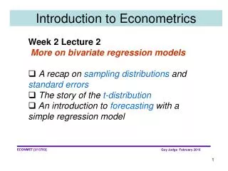
Introduction to Econometrics • Lecture2 • Bivariate regression models • Interpreting least squares regression results: goodness of fit and significance tests • Forecasting with a simple regression model
Recommended reading • DOUGHERTY Introduction to Econometrics Chapter 2 OR • GUJARATI, D N and PORTER, D C Basic Econometrics Chapters 2 & 3
Interpreting basic regression output • Parameter estimates (constant intercept and X coefficient) • Degrees of freedom • The ANOVA table and Sums of Squares • R squared • Standard Error of the Y Estimate (SEE) • Standard error of the X-coefficient • t-values • P values and significance levels • Confidence intervals
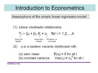
Format of the simple linear regression model • We write the simple linear regression model as Yi = b0 + b1 Xi + ui for i = 1,2,...,n • where Y is the dependent variable • X is the independent variable • and u is the error or disturbance term
Least squares regression results Computer regression software will generate sample values for the least squares estimatesand together with a lot of additional statistical output. Note: we use the term ESTIMATOR for the function (e.g. and ESTIMATE for the actual value that we get when we put sample data on X and Y into this formula.
Some (fictitious) sales-advertising data • Observation Sales(Y) Advertising(X) • 1 36 56.7 • 2 48 63.9 • 3 45 62.7 • 4 40 59.7 • 5 30 55.9 • 6 56 68.7 • 7 63 69.2 • 8 53 65.5 • 9 61 69.4 • 10 68 73.4 • 11 66 74.1 • 12 65 74.4 • NOTE: Both variables are measured in thousands of dollars
The sales-advertising model on a spreadsheet: regression output
Are the coefficient estimates plausible? • The results here show an estimated intercept of -75 and a slope (X) coefficient of just under 2 • What do you think about these values? • Are they significantly different from zero? • How good is the fit?
Analysis of Variance (ANOVA) and Sums of Squares • As you can see from the ANOVA table we can decompose the Total Sum • of Squares (of the dependent variable Y around its mean) into two parts: • the Explained (or Regression) Sum of Squares and • the Residual Sum of Squares. • Total Sum of Squares = • Explained Sum of Squares + Residual Sum of Squares Or in terms of deviations from the mean
Goodness of fit: R squared (the Coefficient of determination) We can now define the Coefficient of Determination or R squared as the proportion of the Total Variation of the dependent variable (around its mean) which can be explained by, or attributed to, the regression. Or, as the second equation has it (1 – the proportion of the variation that is not explained by the regression). R squared is taken as a measure of the “ goodness of fit” of the regression. The closer to 1 is R squared, the better the fit.
Forecasting using the simple regression model (1) Once a model has been estimated (and carefully validated using economic and statistical tests) it can be used for prediction or forecasting. For example our estimated relationship between sales and ads is (approximately) sales = -75 + 1.929 ads + residual We can use this to predict sales for some particular level of advertising, say ads = 70 The disturbance term is assumed to take its expected value so we put the residual = 0.
Forecasting using the simple regression model (2) sales(ads=70) = -75 + 1.9292 * 70 = 60.04 This is just a point forecast. We can create a forecast confidence interval by taking 95% forecast interval = point forecast sF tn-2, 0.025 Here that would give 60.04 2.58097 * 2.228 = 60.04 5.75 i.e. [54.29, 65.79]
Forecasting using the simple regression model (3) This interval is quite large because it is based on a rather small sample. Hence both sF and tn-2, 0.025 will be fairly large. Forecasts based on larger samples will be more precise.