Download
1 / 52
540 likes | 874 Views
Statistics An Introduction. Learning Objectives. 1. Define Statistics 2. Describe the Uses of Statistics 3. Distinguish Descriptive & Inferential Statistics Define Population, Sample, Parameter, & Statistic Identify data types. What is Statistics?.

E N D
Statistics An Introduction
Learning Objectives • 1. Define Statistics • 2. Describe the Uses of Statistics • 3. Distinguish Descriptive & Inferential Statistics • Define Population, Sample, Parameter, & Statistic • Identify data types
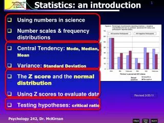
What is Statistics? • The practice (science?) of data analysis • Summarizing data and drawing inferences about the larger population from which it was drawn
Statistical Methods Statistical Methods Descriptive Inferential Statistics Statistics
Descriptive Statistics • 1. Involves • Collecting Data • Presenting Data • Characterizing Data • 2. Purpose • Describe Data $ 50 25 0 Q1 Q2 Q3 Q4 X = 30.5 S2 = 113
Inferential Statistics • 1. Involves • Estimation • Hypothesis Testing • 2. Purpose • Make Decisions About Population Based on Sample Characteristics Population?
Key Terms • 1. Population (Universe) • All Items of Interest • 2. Sample • Portion of Population • 3. Parameter • Summary Measure about Population • 4. Statistic • Summary Measure about Sample • P in Population & Parameter • S in Sample & Statistic
Data Types • Quantitative • Discrete • Continuous • Qualitative • Nominal (categorical) • Ordinal (rank ordered categories)
Sampling • Representative sample • Same characteristics as the population • Random sample • Every subset of the population has an equal chance of being selected
Review • Descriptive vs. Inferential Statistics • Vocabulary • Population • (Random, representative) sample • Parameter • Statistic • Data types
Learning Objectives • 1. Describe Qualitative Data Graphically • 2. Describe Numerical Data Graphically • 3. Create & Interpret Graphical Displays • 4. Explain Numerical Data Properties • 5. Describe Summary Measures • 6. Analyze Numerical Data Using Summary Measures
Student Specializations • Specialization | Freq. Percent Cum. • ---------------+---------------------------------- • HCI | 9 39.13 39.13 • IEMP | 9 39.13 78.26 • LIS | 3 13.04 91.30 • Undecided | 2 8.70 100.00 • ---------------+---------------------------------- • Total | 23 100.00
Undergrad Majors • UG major | Freq. Percent Cum. • --------------------------+----------------------------------- • American Studies | 1 4.76 4.76 • Cog Sci | 1 4.76 9.52 • Comp Sci | 3 14.29 23.81 • Economics | 3 14.29 38.10 • English | 5 23.81 61.90 • Environmental Engineering | 1 4.76 66.67 • Graphic Design | 1 4.76 71.43 • Math | 2 9.52 80.95 • Mechanical Engineering | 1 4.76 85.71 • Nutrition | 1 4.76 90.48 • Sci and Tech Policy | 1 4.76 95.24 • Telecommunications | 1 4.76 100.00 • --------------------------+----------------------------------- • Total | 21 100.00
Favorite Colors • color | Freq. Percent Cum. • ------------+----------------------------------- • black | 2 8.70 8.70 • blue | 12 52.17 60.87 • green | 1 4.35 65.22 • orange | 1 4.35 69.57 • purple | 1 4.35 73.91 • red | 5 21.74 95.65 • white | 1 4.35 100.00 • ------------+----------------------------------- • Total | 23 100.00
Calculus Knowledge • integrals | Freq. Percent Cum. • ------------+----------------------------------- • 1 | 3 13.04 13.04 • 2 | 1 4.35 17.39 • 3 | 11 47.83 65.22 • 4 | 6 26.09 91.30 • 5 | 2 8.70 100.00 • ------------+----------------------------------- • Total | 23 100.00
Student Age (Reported) Data • Stem-and-leaf plot for age • 2* | 22233444555777899 • 3* | 01257 • 4* | • 5* | • 6* | • 7* | 6
Starting Salaries (in $K) • 3* | 8 • 4* | 000025 • 5* | 0000 • 6* | 0000005 • 7* | 5 • 8* | 0
Thinking Challenge $400,000 $70,000 $50,000 ... employees cite low pay -- most workers earn only $20,000. ... President claims average pay is $70,000! $30,000 $20,000
Standard Notation Measure Sample Population Mean x Stand. Dev. s 2 2 Variance s Size n N
Numerical Data Properties Central Tendency (Location) Variation (Dispersion) Shape
Numerical DataProperties & Measures Numerical Data Properties Central Variation Shape Tendency Mean Range Skew Interquartile Range Median Mode Variance Standard Deviation
Numerical DataProperties & Measures Numerical Data Properties Central Variation Shape Tendency Mean Range Skew Interquartile Range Median Mode Variance Standard Deviation
What’s wrong with this? • Measurements 1 4 2 9 8 • Middle measurement is 2, so that’s the median X i X X X 1 2 n i 1 X n n
Ages • Mean = 29 • Median = 27 • 2* | 22233444555777899 • 3* | 01257 • 4* | • 5* | • 6* | • 7* | 6
Summary of Central Tendency Measures Measure Equation Description Mean Balance Point X / n i Median ( n +1) Position Middle Value 2 When Ordered Mode none Most Frequent
Numerical DataProperties & Measures Numerical Data Properties Central Variation Shape Tendency Mean Range Skew Median Interquartile Range Mode Variance Standard Deviation
Shape • 1. Describes How Data Are Distributed • 2. Measures of Shape • Skew = Symmetry Left-Skewed Symmetric Right-Skewed Mean Median Mode Mean = Median = Mode Mode Median Mean
Numerical DataProperties & Measures Numerical Data Properties Central Variation Shape Tendency Range Mean Skew Interquartile Range Median Mode Variance Standard Deviation
Quartiles • 1. Measure of Noncentral Tendency • 2. Split Ordered Data into 4 Quarters • 3. Position of i-th Quartile 25% 25% 25% 25% Q1 Q2 Q3 i (n 1) Positionin g Point of Q i 4
Ages • Range • Quartiles • 2* | 22233444555777899 • 3* | 01257 • 4* | • 5* | • 6* | • 7* | 6
Quartiles: 24, 27, 30 Inner fences: (15,39) Outer fences: (6, 48) Quartiles: 41K, 50K, 60K Inner fences: ?? Outer fences: ?? Box Plots - Age and Salary
Variance & Standard Deviation • 1. Measures of Dispersion • 2. Most Common Measures • 3. Consider How Data Are Distributed • 4. Show Variation About Mean (X or ) X = 8.3 4 6 8 10 12
Sample Variance Formula n 2 n - 1 in denominator! (Use N if Population Variance) X) (X i 2 i 1 S n 1 2 2 2 (X X) (X X) ... (X X) 1 2 n n 1
Empirical Rule • If x has a “symmetric, mound-shaped” distribution • Justification: Known properties of the “normal” distribution, to be studied later in the course
Preview of Statistical Inference • You observe one data point • Make hypothesis about mean and standard deviation from which it was drawn • Empirical Rule tells you how (un)likely the data point is • If very unlikely, you are suspicious of the hypothesis about mean and standard deviation, and reject it
2 X X i n 1 2 X i X N Summary of Variation Measures Measure Equation Description X - X Total Spread Range largest smallest Q - Q Spread of Middle 50% Interquartile Range 3 1 Dispersion about Standard Deviation Sample Mean (Sample) Dispersion about Standard Deviation Population Mean (Population) 2 Squared Dispersion Variance ( X - X ) i about Sample Mean (Sample) n - 1