Download
1 / 23
230 likes | 252 Views
Learn about binomial and geometric distributions, probability calculations, parameters, calculator functions, mean, variance, and normal approximation. Explore examples, exercises, and the importance of these distributions in statistical inference.

E N D
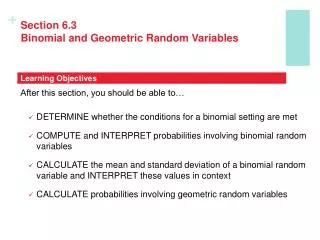
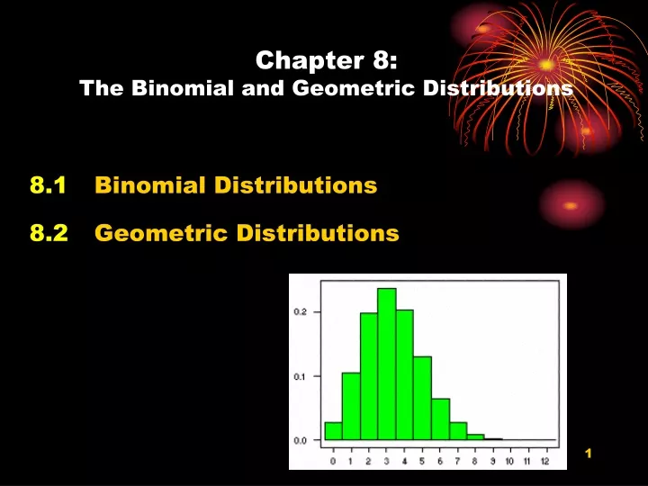
Chapter 8:The Binomial and Geometric Distributions 8.1 Binomial Distributions 8.2 Geometric Distributions
Let me begin with an example… • My best friends from Kent School had three daughters. What is the probability of having 3 girls? • We calculate this to be 1/8, assuming that the probabilities of having a boy and having a girl are equal. • But the point in beginning with this example is to introduce the binomial setting.
The Binomial Setting (p. 439) • Let’s begin by defining X as the number of girls. • This example is a binomial setting because: • Each observation (having a child) falls into just one of two categories: success or failure of having a girl. • There is a fixed number of observations (n). • The n observations are independent. • The probability of success (p) is the same for each observation.
Binomial Distributions • If data are produced in a binomial setting, then the random variable X=number of successes is called a binomial random variable, and the probability distribution of X is called a binomial distribution. • X is B(n,p) • n and p are parameters. • n is the number of observations. • p is the probability of success on any observation.
How to tell if we have a binomial setting … • Examples 8.1-8.4, pp. 440-441 • Exercise 8.1, p. 441
Binomial Probabilities—pdf • We can calculate the probability of each value of X occurring, given a particular binomial probability distribution function. • 2nd (VARS) 0:binompdf (n, p, X) • Try it with our opening example: • What is the probability of having 3 girls? • Example 8.5, p. 442 • Note conclusion on p. 443
Binomial Probabilities—cdf • Example 8.6, p. 443 • We can use a cumulative distribution function (cdf) to answer problems like this one. • Binomcdf (n, p, X)
Problems • 8.3 and 8.4, p. 445
Binomial Formulas • We can use the TI-83/84 calculator functions binompdf/cdf to calculate binomial probabilities, as we have just discussed. • We can also use binomial coefficients (p. 447). Read pp. 446-448 carefully to be able to use this alternate approach.
Homework • Read through p. 449 • Exercises: • 8.6-8.8, p. 446 • 8.12-8.13, p. 449
Mean and Standard Deviation fora Binomial Random Variable • Formulas on p. 451: • Now, let’s go back to problem 8.3, p. 445. Calculate the mean and standard deviation and compare to the histogram created.
Normal Approximation to Binomial Distributions • As the number of trials, n, increases in our binomial settings, the binomial distribution gets close to the normal distribution. • Let’s look at Example 8.12, p. 452, and Figure 8.3. • I show this because it begins to set the stage for very important concept in statistical inference—The Central Limit Theorem. • Because of the power of our calculators, however, I recommend exact calculations using binompdf and binomcdf for binomial distribution calculations.
Rules of Thumb • See box, top of page 454.
Problems • 8.15 and 8.17, p. 454 • 8.19, p. 455 • 8.27, 8.28, and 8.30, p. 461
Homework • Reading, Section 8.2: pp. 464-475 • Review: • Conditions for binomial setting • Compare to conditions for geometric setting • What’s the key difference between the two distributions? • Test on Monday
8.2 Geometric Distributions • I am playing a dice game where I will roll one die. I have to keep rolling the die until I roll a 6, then the game is over. • What is the probability that I win right away, on the first roll? • What is the probability that it takes me two rolls to get a 6? • What is the probability that it takes me three rolls to get a 6?
The Geometric Setting • This example is a geometric setting because: • Each observation (rolling a die) falls into just one of two categories: success or failure. • The probability of success (p) is the same for each observation. • The observations are independent. • The variable of interest is the number of trials required to obtain the first success.
Calculating Probability • For a geometric distribution, the probability that the first success occurs on the nth trial is: • Let’s look at Example 8.16, p. 465, and then the example calculations below that example for Example 8.15. • Why the name “geometric” for this distribution? • See middle of page 466.
“Calculator Speak” • Notice that we do not have an “n” present in the following calculator commands … that’s the point of a geometric distribution!
Exercises:8.38, p. 4688.43 (b&c), p. 474 -- See example 8.15, p. 465
Homework • Read through the end of the chapter. • Problems: • 8.36, p. 463 • 8.39, p. 468 • 8.46, p. 474 • 8.55 and 8.56, p. 479 • 8.1-8.2 Quiz Friday
Chapter 8 Review Problems • pp. 480-482: • 8.60 • 8.61 • 8.62 • 8.63