Download

1 / 78
950 likes | 1.35k Views
Power Analysis. An Overview. Power Is. The conditional probability that one will reject the null hypothesis given that the null is really false by a specified amount and given certain other specifications such as sample size and the criterion of statistical significance (alpha). .

E N D
Power Analysis An Overview
Power Is • The conditional probability • that one will reject the null hypothesis • given that the null is really false • by a specified amount • and given certain other specifications such as sample size and the criterion of statistical significance (alpha).
A Priori Power Analysis • You want to find how many cases you will need to have a specified amount of power given • a specified effect size • the criterion of significance to be employed • whether the hypotheses are directional or nondirectional • A very important part of the planning of research.
A Posteriori Power Analysis • You want to find out what power would be for a specified • effect size • sample size • and type of analysis • Best done as part of the planning of research. • could be done after the research to tell you what you should have known earlier.
Retrospective Power Analysis • Also known as “observed power.” • What would power be if I were to • repeat this research • with same number of cases etc. • and the population effect size were exactly what it was in the sample in the current research • Some stat packs (SPSS) provide this.
Hoenig and Heisey • The American Statistician, 2001, 55, 19-24 • Retrospective power asks a foolish question. • It tells you nothing that you do no already know from the p value. • After the research you do not need a power analysis, you need confidence intervals for effect sizes.
One Sample Test of Mean • Experimental treatment = memory drug • H0: µIQ 100; σ = 15, N = 25 • Minimum Nontrivial Effect Size (MNES) = 2 points. • Thus, H1: µ = 102.
= .05, MNES = 2, Power = ? • Under H0, CV = 100 + 1.645(3) = 104.935 • will reject null if sample mean 104.935 • Power = area under H1 104.935 • Z = (104.935 102)/3 = 0.98 • P(Z > 0.98) = .1635 • = 1 - .16 = .84 • Hope you like making Type II errors.
= .05, ES = 5, Power = ? • What if the Effect Size were 5? • H1: µ = 105 • Z = (104.935 105)/3 = 0.02 • P(Z > 0.02) = .5080 • It is easier to find large things than small things.
H0: µ = 100 (nondirectional) • CVLower = 100 1.96(3) = 94.12 or less • CVUpper = 100 + 1.96(3) = 105.88 or more • If µ = 105, Z = (105.88 105)/3 = .29 • P(Z > .29) = .3859 • Notice the drop in power. • Power is greater with directional hypothesis IF you can correctly PREdict the direction of the effect.
Type III Error • µ = 105 but we happen to get a very low sample mean, at or below CVLower. • We would correctly reject H0 • But incorrectly assert the direction of effect. • P(Z < (94.12 105)/3) = P(Z < 3.63), which is very small.
H0: µ = 100, N = 100 • Under H0, CV = 100 + 1.96(1.5) = 102.94 • If µ = 105, Z = (102.94 105)/1.5 = -1.37 • P(Z > -1.37) = .9147 • Anything that reduces the SE increases power (increase N or reduce σ)
Reduce to .01 • CVUpper = 100 + 2.58(1.5) = 103.87 • If µ = 105, Z = (103.87 105)/1.5 = -0.75 • P(Z > 0.75) = .7734 • Reducing reduces power, ceteris paribus.
z versus t • Unless you know σ (highly unlikely), you really should use t, not z. • Accordingly, the method I have shown you is approximate. • If N is not small, it provides a good approximation. • It is primarily of pedagogical value.
Howell’s Method • The same approximation method, but • You don’t need to think as much • There is less arithmetic • You need his power table
IQ problem, minimum nontrivial effect size at 5 IQ points, d = (105 100)/15 = 1/3. • with N = 25, = 1/3 5 = 1.67. • = (1/3)5 = 1.67. • Using the power table in our text, for a .05 two-tailed test, power = 36% for a of 1.60 and 40% for a of 1.70 • power for = 1.67 is 36% + .7(40% 36%) = 38.8%
I Want 95% Power • From the table, is 3.60. • If I get data on 117 cases, I shall have power of 95%. • With that much power, if I cannot reject the null, I can assert its near truth.
The Easy Way: GPower • Test family: t tests • Statistical test: Means: Difference from constant (one sample case) • Type of power analysis: Post hoc: Compute achieved power – given α, sample size, and effect size • Tails: Two • Effect size d: 0.333333 (you could click “Determine” and have G*Power compute d for you) • α error prob: 0.05 • Total sample size: 25 • This is NOT an approximation, it uses the t distribution.
Significant Results, Power = 36% • Bad news – you could only get 25 cases • Good news – you got significant results • Bad news – the editor will not publish it because power was low. • Duh. Significant results with low power speaks to a large effect size. • But also a wide confidence interval.
Nonsignificant Results • Power = 36% • You got just what was to be expected, a Type II error. • Power = 95% • If there was anything nontrivial to be found, you should have found it, so the effect is probably trivial. • The confidence interval should show this.
I Want 95% Power • How many cases do I need?
Sensitivity Analysis • I had lots of data, N = 1500, but results that were not significant. • Can I assert the range null that d 0. • Suppose that we consider d 0 if -0.1 d +0.1. • For what value of d would I have had 95% power?
If the effect were only .093, I would have almost certainly found it. • I did not find it, so it must be trivial in magnitude • I’d rather just compute a CI.
Two Independent Samples Test of Means • Effective sample size, . • The more nearly equal n1 and n2, the greater the effective sample size. • For n = 50, 50, it is 50. For n =10, 90, it is 18.
Howell’s Method: Aposteriori • n1 = 36, n2= 48, effect size = 40 points,SD = 98 • From the power table, power = 46%.
I Want 80% Power • For effect size d = 1/3. • From power table, = 2.8 with alpha .05 • I plan on equal sample sizes. • Need a total of 2(141) = 282 subjects.
G*Power • We have 36 scores in one group and 48 in another. • If µ1 - µ2 = 40, and σ = 98, what is power?
I Want 80% Power • n1 = n2 = ? for d = 1/3, = .05, power = .8. • You need 286 cases.
Allocation Ratio = 9 • n1/n2 = 9. How many cases needed now? • You need 788 cases!
Two Related Samples, Test of Means • Is equivalent to one sample test of null that mean difference score = 0. • With equal variances, • The greater , the smaller the SE, the greater the power.
dDiff • Adjust the value of d to take into account the power enhancing effect of this design.
Howell’s Method: A Posteriori • Effect size = 20 points: • Cortisol level when anxious vs. when relaxed • σ1 = 108, σ2 = 114 • = .75 • N = 16 • Power = ?
Howell’s Method • Pooled SD = • d = 20/111 = .18. • From the power table, power = 17%.
G*Power • Dependent means, post hoc. • Set the total sample size to 16. • Click on “Determine.” • Select “from group parameters.” • Calculate and transfer to main window.
I Want 95% Power • You need 204 subjects.
Type III Errors • You have correctly rejected H0: µ1= µ2. • Which µ is greater? • You conclude it is the one whose sample mean was greater. • If that is wrong, you made a Type III error. • This probability is included in power. • To exclude it, see http://core.ecu.edu/psyc/wuenschk/StatHelp/Type_III.htm
Bivariate Correlation/Regression • H0: Misanthropy-AnimalRights = 0 • For power = .95, = .05, = .2, N = ?
Steiger & Fouladi’s R2 • Option, Sample size calculation • K = 2, = .05, 2 = .04, P = .95, Go, N = 319.
N = 314 or 319 ? • Why different answers to same question? • My guess is • GPower assumes a regression analysis (fixed X, random Y – “point biserial model”) • R2 assumes a correlation model (both X and Y random) • or maybe just different algorithms
One-Way ANOVA, Independent Samples • f is the effect size statistic. Cohen considered .1 to be small, .25 medium, and .4 large. • In terms of 2, this is 1%, 6%, 14%.
Comparing three populations on GRE-Q • Minimum nontrivial effect size is if each ordered mean differs from the next by 20 points (about 1/5 SD). • (µj - µ)2 = 202 + 02 + 202 = 800
Analysis of Covariance • Adding covariates to the ANOVA model can increase power. • If they are well correlated with the dependent variable. • Adjust the f statistic this way, where r is the corr between covariate(s) and Y.
k = 3, f = .1, power = .95, N = ? • Ouch, that is a lot of data we need here.