Download
1 / 16
280 likes | 967 Views
Quadrature Amplitude Modulation (QAM) format. Features of QAM format:. Two carriers with the same frequency are amplitude-modulated independently. The phase of the two carriers is 90 deg. shifted each other.

E N D
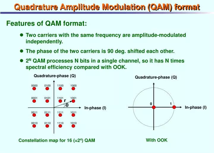
Quadrature Amplitude Modulation (QAM) format Features of QAM format: • Two carriers with the same frequency are amplitude-modulated independently. • The phase of the two carriers is 90 deg. shifted each other. • 2NQAM processes N bits in a single channel, so it has N times spectral efficiency compared with OOK. Quadrature-phase (Q) Quadrature-phase (Q) 0000 0100 1100 1000 0001 0101 1101 1001 1 0 In-phase (I) In-phase (I) 0011 0111 1111 1011 0010 0110 1110 1010 With OOK Constellation map for 16 (=24) QAM
Various modulation formats for microwaves and their spectral efficiencies [1] Large Small Fixed amplitude Amplitude change (-1.6 dB) Quadrature modulation type ASK type MSK type FSK type PSK type Shannon limit 1024 256 64 16 ・16 QAM • Multi-level FSK • Quadrature • modulation • Associated • quadrature • modulation M-QAM C/W (bit/s/Hz) 4 ・64 QAM • Duobinary • FSK Correlation PSK Coded Satellite communication ・256 QAM Adoption of coding technique Mobile communication Coded modulation Fixed wireless communication Eb/N0 (dB) C: Channel capacity(bit/s), W: Bandwidth (Hz) Eb/N0: Energy to noise power density ratio per bit Eb/N0 at BER = 10-4 is shown assuming synchronous detection Increase in power efficiency Increase in spectral efficiency Modulation schemes and their application fields Spectral efficiency of various modulation schemes [1] Y. Saito, “Modulation and demodulation in digital wireless communication,” IEICE (in Japanese)
Integrated global network 100 Gb/s~1 Tb/s per wavelength Regional IP backbone network 10 Gb/s~40 Gb/s per wavelength User access network 10 Mb/s~1 Gb/s Advantages of QAM optical transmission Microwave transmission Drawbacks of QAM wireless or metallic cable transmission: Obstacle Transmitted point Fading noise caused by obstacles Narrow bandwidth transmission Free space Received point Metallic cable Optical fiber transmission Advantages of QAM optical transmission: No fading noise in optical fibers Broad bandwidth transmission
Configuration for QAM coherent transmission IF signal fIF=fs- fL Optical fiber fs Coherent light source Demodulator PD QAM modulator fL Local oscillator (LO) Optical phase- locked loop (OPLL) circuit Key components of QAM coherent transmission: - Coherent light source: C2H2 frequency-stabilized laser - QAM modulator: Single sideband (SSB) modulator - OPLL circuit: Tunable tracking laser as an LO - Demodulator: Digital demodulator using a software (DSP)
1.5 GHz Reflection [dB] Wavelength [nm] A C2H2 frequency-stabilized fiber laser[1] Feedback Circuit Low Pass Filter 1.48 mm LD VPZT PZT EDF WDM Electrical Amp Cavity Length ~ 4 m (FSR= 49.0 MHz) PM- FBG[2] DBM Circulator MLP Electrical Amp 80/20 Coupler Phase Sensitive Detection Circuit PD Coupler 13C2H2 Cell LN Frequency Modulator 1.54 mm Optical Output (No Frequency Modulation) Laser Frequency Stabilization Unit Single-frequency Fiber Ring Laser • Frequency stability: 2x10-11 • Line width: 4 kHz [1] K. Kasai et al., IEICE ELEX., vol. 3, 487 (2006). [2] A. Suzuki et al., IEICE ELEX., vol. 3, 469 (2006).
QAM modulator[1] Electrical magnitude of optical signal I data RFA: F1(t)+DCA time MZA MZC Optical input Optical output MZB Electrical magnitude of optical signal p/2 DCC Q data RFB: F2(t)+DCB time MZ: Mach-Zehnder interferometer Configuration of QAM modulator I data Q data DCC [1] S. Shimotsu et al., IEEE Photon. Technol. Lett., vol. 13, 364 (2001).
-40 Phase error: 0.3 deg. -60 -80 SSB phase noise [dBc/Hz] -100 -120 -140 10 Hz 1 MHz Frequency offset SSB phase noise spectrum OPLL circuit with a tunable fiber laser as an LO[1] Resolution: 10 Hz RF spectrum analyzer 500 Hz Less than 10 Hz IF signal: fIF=fs-fL Loop filter1 (Fast operation: 1 MHz) DBM fs PD fsyn Loop filter2 (Slow operation: 10 kHz) Synthesizer to PZT fL LO IF signal spectrum to LN phase modulator Tunable fiber laser - Linewidth: 4 kHz - Bandwidth of frequency response:1.5 GHz [1] K. Kasai et al., IEICE ELEX., vol. 4, 77 (2007).
LPF LPF Configuration of digital demodulator (Software Processing) DSP I(t) QAM Signal S(t) = I(t)cos(wIFt+f0) -Q(t)sin(wIFt+f0) 2cos(wIFt+f) Clock signal Save to file Decode A/D 0, 1, 0, 0, • • • p/2 -2sin(wIFt+f) Q(t) Bit Error Rate Measurement Accumulation of QAM Data Signal Digital Demodulation Circuit Our system operates in an off-line condition by using softwares.
I QAM data signal Pilot Intensity 2.5 GHz Q Optical Frequency Polarization-multiplexed 1 Gsymbol/s, 64 QAM (12 Gbit/s) coherent optical transmission system[1] Arbitrary Waveform Generator Delay Line QAM( ) I ⊥ QAM Modulator Arbitrary Waveform Generator Q QAM(//) Optical Filter (~ 5nm) QAM Modulator Att PBS C2H2 Frequency-Stabilized Fiber Laser OFS PC DSF 75 km DSF 75 km Pilot EDFA (MUX) (fOFS =2.5 GHz) 2 GHz FBG IF Signal fIF=fsyn+fOFS=4 GHz Digital Signal Processor A/D PD Att PBS ( or ) (DEMUX) DBM PD EDFA: Erbium-doped Fiber Amplifier PC: Polarization Controller OFS: Optical Frequency Shifter PBS: Polarization Beam Splitter DSF: Dispersion-shifted Fiber FBG: Fiber Bragg Grating PD: Photo-detector DBM: Double Balanced Mixer (fsyn= 1.5 GHz) Feedback Circuit Synthesizer LO [1] M. Nakazawa, et al., OFC2007, PDP26 (2007).
(//) (//) (//) Electrical spectrum of IF signal ( ) (//) ( ) Demodulation bandwidth Demodulation bandwidth 2 GHz 2 GHz (a) Orthogonal polarization (b) Parallel polarization
Experimental result for polarization-multiplexed 1 Gsymbol/s, 64 QAM (12 Gbit/s) transmission over 150 km Constellation diagram Eye pattern (I) Eye pattern (Q) (a) Back-to-back (Received power: -29 dBm) (b) 150 km transmission for orthogonal data (Received power: -26 dBm) (c) 150 km transmission for parallel data (Received power: -26 dBm)
Transfer function Impulse response Bandwidth narrowing f f Data signal spectrum Improvement of spectral efficiency by using a Nyquist filter[1] Nyquist filter: Bandwidth reduction of data signal without intersymbol interference [1] H. Nyquist, AIEEE Trans, 47 (1928).
( ) ( ) (//) Electrical spectrum of IF data signal ( ) (//) ( ) Demodulation bandwidth Demodulation bandwidth 2 GHz 1.5 GHz (a) Without Nyquist filter (b) With Nyquist filter Roll off factor: 0.35
Experimental result for polarization-multiplexed 1 Gsymbol/s, 64 QAM (12 Gbit/s) transmission over 150 km[1] Q Q Q Constellation diagram Eye pattern (I) Eye pattern (Q) (a) Back-to-back (Received power: -29 dBm) (b) 150 km transmission for orthogonal data (Received power: -26 dBm) (c) 150 km transmission for parallel data (Received power: -26 dBm) [1] K. Kasai et al., OECC2007, PDP, PD1-1 (2007).
Orthogonal polarization (Back-to-back) Orthogonal polarization (150 km transmission) Parallel polarization (Back-to-back) Parallel polarization (150 km transmission) Bit error rate (BER) characteristics 3 dB
Conclusion • Two emerging optical transmission technologies were described. • (1) Ultrahigh-speed OTDM transmission • 160 Gbit/s-1,000 km transmission was successfully achieved by combing DPSK and time-domain OFT. • OFT has crucial potential especially for high bit rate, thus it is expected to play an important role for OTDM transmission at 320 Gbit/s and even faster. • (2) Coherent QAM transmission • We have successfully transmitted a polarization-multiplexed 1 Gsymbol/s, 64 QAM (12 Gbit/s) coherent optical signal over 150 km within an optical bandwidth of 1.5 GHz using a Nyquist filter. • Thus, a spectral efficiency of 8 bit/s/Hz has been achieved in a single-channel.