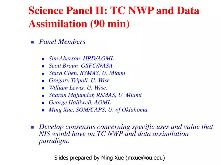
Science Panel II: TC NWP and Data Assimilation (90 min)

1. Science Panel II: TC NWP and Data Assimilation (90 min) • Panel Members • Sim Aberson HRD/AOML • Scott Braun GSFC/NASA • Shuyi Chen, RSMAS, U. Miami • Gregory Tripoli,U. Wisc. • William Lewis, U. Wisc. • Sharan Majumdar, RSMAS, U. Miami • George Halliwell, AOML • Ming Xue, SOM/CAPS, U. of Oklahoma. • Develop consensus concerning specific uses and value that NIS would have on TC NWP and data assimilation paradigm. Slides prepared by Ming Xue (mxue@ou.edu)

2. Specific Questions: • Given that operational TC NWP model(s) are expected to be running at cloud-resolving resolutions (~km) and possibly in ensemble mode during the lifetime of the NIS, how will its observations facilitate the initialization of TCs and their precursors via advanced data assimilation? • What are the most desirable observed parameters (e.g., radial velocity, reflectivity, polarimetric variables, Doppler spectra/spectrum width, differential reflectivity) and what unique information do they provide for the cloud-resolving TC NWP purpose? • What unique information will NIS provide to enhance data assimilation for TCs in global and other non-TC specific models that will most likely to be running at non-cloud-resolving resolutions? • What is the expected duration of NIS impact on both deterministic and probabilistic TC forecasts? • What are the expected impacts of NIS observations on the overall intensity/structure prediction problem?

3. Specific Questions - continued • Given that operational TC NWP model(s) are expected to be running at What are the expected impacts of NIS observations on TC surge and hydrological forecasting derived from TC model forecasts? • Within the proposed technological constraint (~spiral scans of 5000 km diameter area every hour, at 12 km resolution without over-sampling), what might be the preferred scanning configurations for the cloud-resolving TC NWP purpose? • Should or can NIS operate in coarse grain (e.g., tracking TC vortex) or fine-grain (e.g., changing scanning configurations for different parts of the TC on the fly and choosing scanning modes based on expected TC development) adaptive scanning mode? What happens when multiple TCs are in view?

4. Additional charge: • Given proposed NIS instrument design (i.e., frequency, Doppler acuity, polarimetric diversity, resolution, scan strategy, orbit) and issues relevant to future TC NWP and data assimilation (i.e., cloud resolving deterministic and probabilistic models), develop consensus on: • aspects of design that are particularly useful, • critical weaknesses that must be addressed, • enhancements to design that should be considered.

5. NWP should be here! • Properly initialized NWP models with complete, dynamically consistent IC should out-perform extrapolation/statistical nowcasting models from time zero • Current ICs of TC prediction are no where close to being complete/dynamically consist  spin-up problem Nowcasting v.s. Short-range NWP of Convection/Precipitation • The quoted NWP models are not initialized with radar and/or other high-res data and/or their resolution is too low (Jim Wilson 2006, US-Korea Workshop)

6. CAPS and CASA • CAPS was established as one of the 1st NSF Science & Technology Centers in 1989 at University of Oklahoma • CAPS's mission was and still is to develop and demonstrate methods/techniques for the numerical analysis and prediction of high-impact local weather conditions, with emphasis on the assimilation of observations from Doppler radars and other advanced in-situ and remote sensing systems. • CASA – NSF ERC for Collaborative Adaptive Sensing of Atmosphere. Develop low-cost dense network of radars to dynamically adaptively sensing the lower atmosphere.

7. US WSR-88D (NETRAD) Doppler Radar Network

8. WSR-88D radar coverage at 1 km AGL - low-level coverage is poor

9. Radar Data Assimilation • Advanced data assimilation techniques essential for radar data – a problem of both analysis and retrieval! • Vr and Z only, more with polarimetric radars, usually only in precipitation regions • All other state variables have to be ‘retrieved’ • Leading methods: 3DVAR, 4DVAR and EnKF methods

10. NIS Data • NIS Data, while unprecedented, and extremely important in filling the ‘gap’, are by no means complete (no direct observations of state variables) • Advanced 4-D data assimilation (DA) methods essential • Need to closely couple with model dynamics and physics

11. DA cycles on 1-km Grid 3DVAR+Cloud Analysis Forecast 2030 UTC 2140 UTC 4 nested grids May 8th, 2003 OKC tornado case

12. ARPS 1-km-grid forecast using 3DVAR + Cloud Analysis cycles over 1 hour Reflectivity at 1.45º elevation 30-min forecast 40-min forecast

13. 50-m Grid Forecast v.s. Observation Forecast Low-level Reflectivity Observed Low-level Reflectivity 43 minute forecast

14. Ensemble Kalman Filter DA Method Obs Obs t+1 t t=0 Assimilation Assimilation

15. For radar data assimilation Radar data: Vr only @ Z>10dBZ Vr@ Z>10dBZ & Z K: Kalman gain calculated from background and obs error covariances (Tong and Xue 2005 MWR, Xue et al. 2006, JTech.) Very good results with OSSEs

16. Low level cold pool (q') and reflectivity Truth Vr Vr & Z

17. Analysis of Microphysical Variables at T=65 min Truth Vr + Z qc, qr, qi, qs, qh

18. Ensemble forecast • Ensembles of forecasts (e.g., 3 hourly) are launched periodically from the ensemble analyses produced at much shorter intervals (e.g., every 15 minutes) • Probabilistic info is provided by the ensembles • Optimal scanning strategies can be chosen to maximize future forecast error reduction, using, e.g., ETKF method.

19. Capturing and Variationally Analyzing Tornadic Circulation via Azimuthal Over-sampling (2 degree beams) (Xue et al 2007 JTech) 0.125o 1o 2o Sampled Vr with azimuthal increments of (a) 2o, (b) 1o and (c) 0.125o (c) • Over-sampling alone, without wind retrieval, is not much of a help beyond a factor of two over-sampling • Variational ‘de-convolution’ for sub-beam width structures

20. Importance of Observation Operator when observations are integrated quantities (e.g., radar Z and Vr, sat. radiance data) Sample Volume Beam pattern weighted Vr sampling Illustration of the simulation of radial velocity data from a gridded wind field.

21. Impact of azimuthal increments of sampling u v wind truth “truth” & analyses from radial velocity data sampled at azimuthal increments of 0.125oand 2o O/S 0.125o CC=0.9 Beamwidth = 2o Distance of radars = 15 km N/OS 2o CC=0.7

22. 8 times oversampling with KOUN 35 60 no oversampling u v V Vr from KTLX and KOUN for May 10th, 2003 OKC tornado case KTLX KOUN .125o inc. KOUN 1.0o inc.

23. Comments • The observation operator did not include reflectivity weighting • Reflectivity weighting essential for 12 km beams • Attenuation is not considered • Attenuation can and should be built in the observation operator and used in DA system!

24. Simulated reflectivity before and after attenuation (2nd tilt) for a supercell storm

25. EnKF Assimilation without attenuation correction Data without attenuation (black) Data with attenuation, no attenuation correction

26. Assimilation with attenuation correction Data with attenuation, attenuation correction is included in the forward operator (red) Data without attenuation (black)

27. Comments • Complete attenuation still a problem – complete loss of signal (single 94 GHz probably not desirable) – low level obs most important. • Both attention and reflectivity strongly dependent on microphysics (phase, size and shape of hydrometeors) – need better (e.g., two-moment) MP schemes • Fall speeds of hydrometeors are equally strongly dependent on MP – can contaminating the most-important vertical velocity information. • DSD info via dual-frequency reflectivity/attenuation ratio may be valuable • Reflectivity weight depends on model-resolved convective cell structures and distribution • Model forecast used as the analysis background cannot deviate too much from the truth – hence the need for cycle length < ½ cell life cycle • Important to retain sub-beam-scale structures in the background forecast rather than suppressing them in the analysis process – otherwise spinup problem remains (though to a less extent than when without NIS at all)

28. 2 hr forecast @ Dx=3km for May 3, 1999 OKC F-5 Tornado CaseBase Reflectivity and qv at 0000 UTC Lin Lin w/ reduced N0r WSM6 WSM6 (diag N0r) MY3 = Milbrandt and Yau 3-moment scheme MY1 MY2 MY3

29. Single-Sounding Simulations (Dx=500 m) Surface Reflectivity and qv at 1 hr

30. Comments • Need additional and more sophisticated OSSEs (Observing System Simulation Experiments) that • realistically simulate observation data from sub-km resolution simulations (can include side lobes) • assimilate the data at expected TC NWP resolutions (~ 1 km) • assess impact and help refine NIS design and scanning strategies • yes,prediction model needs to be an integral part of the signal-processing (from Chandra - can't believe it came from a radar engineer!)

31. One of such examples See also Simone Tanelli and Mike Biggerstaff’s presentations.

32. Scanning Strategies • 15-min volume scans (4 times the frequency) • A factor of 2 over-sampling (~6 km increments, 4 times number of samples) • 1250 km diameter region for established TCs (1/16th scan area) • Achievable without second arm • Data assimilated continuously as they come in, not necessarily at 15-min discrete intervals • Assimilated together with e.g., airborne radar data that better capture horizontal winds, and other data defining environmental wind, T, and qv. • Cycles startied from pre-genesis stage • Larger area without over-sampling at pre- and genesis stages? • Fine-grained adaptive sampling?

33. Expected length of impact at individual cell, organized rainband/eyewall and TC scales, on deterministic and probabilistic forecasting? • At individual cell level, no more 1 hour • At rainband/eyewall scale ~ a few to tens of hours? • At TC scale – several days? Definitely the accumulated impact via continuous cycles • Difference between deterministic and probabilistic forecasts?

34. Data Quality Info/Error Estimate? • Spectrum width info useful in DA? • What error estimation can be provided for the data? Is signal-to-noise ratio available for estimating sampling errors? • Need to define R – obs error covariance matrix – do not want correlated errors. • Other QC issues (unfolding, clutter removal, attenuation correction, beam pattern uncertainty, etc.)